A new method for solving the mgrlw equation using a base of quintic B-Spline
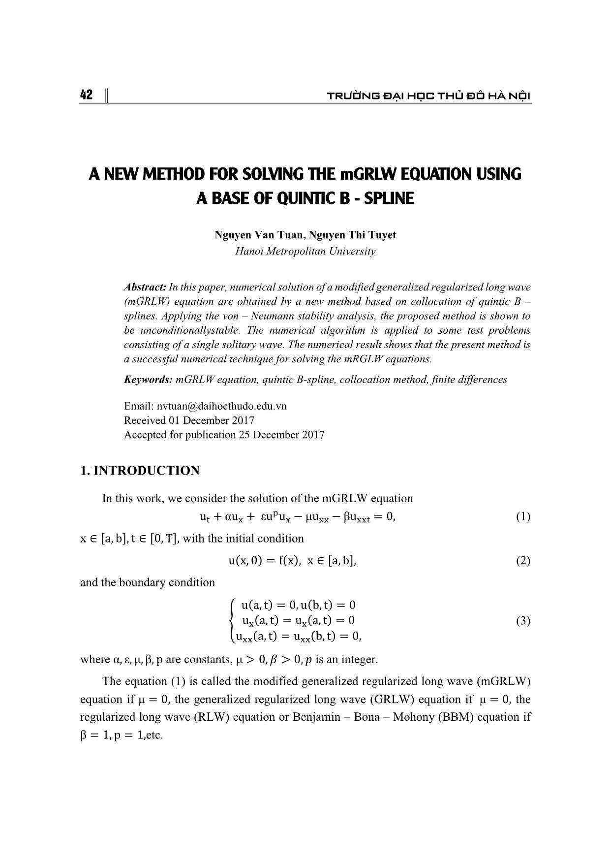
In this paper, numerical solution of a modified generalized regularized long wave
(mGRLW) equation are obtained by a new method based on collocation of quintic B –
splines. Applying the von – Neumann stability analysis, the proposed method is shown to
be unconditionallystable. The numerical algorithm is applied to some test problems
consisting of a single solitary wave. The numerical result shows that the present method is
a successful numerical technique for solving the mRGLW equations.
Trang 1
Trang 2
Trang 3
Trang 4
Trang 5
Trang 6
Trang 7
Trang 8
Trang 9
Trang 10
Tải về để xem bản đầy đủ
Bạn đang xem 10 trang mẫu của tài liệu "A new method for solving the mgrlw equation using a base of quintic B-Spline", để tải tài liệu gốc về máy hãy click vào nút Download ở trên
Tóm tắt nội dung tài liệu: A new method for solving the mgrlw equation using a base of quintic B-Spline
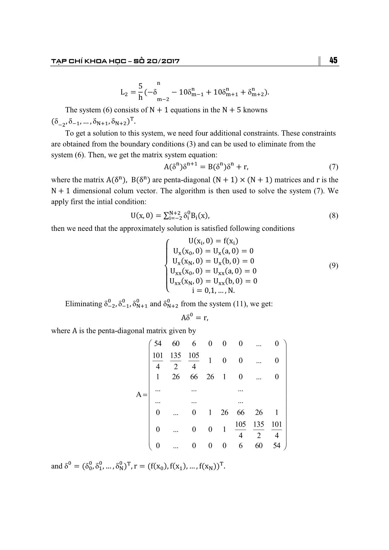
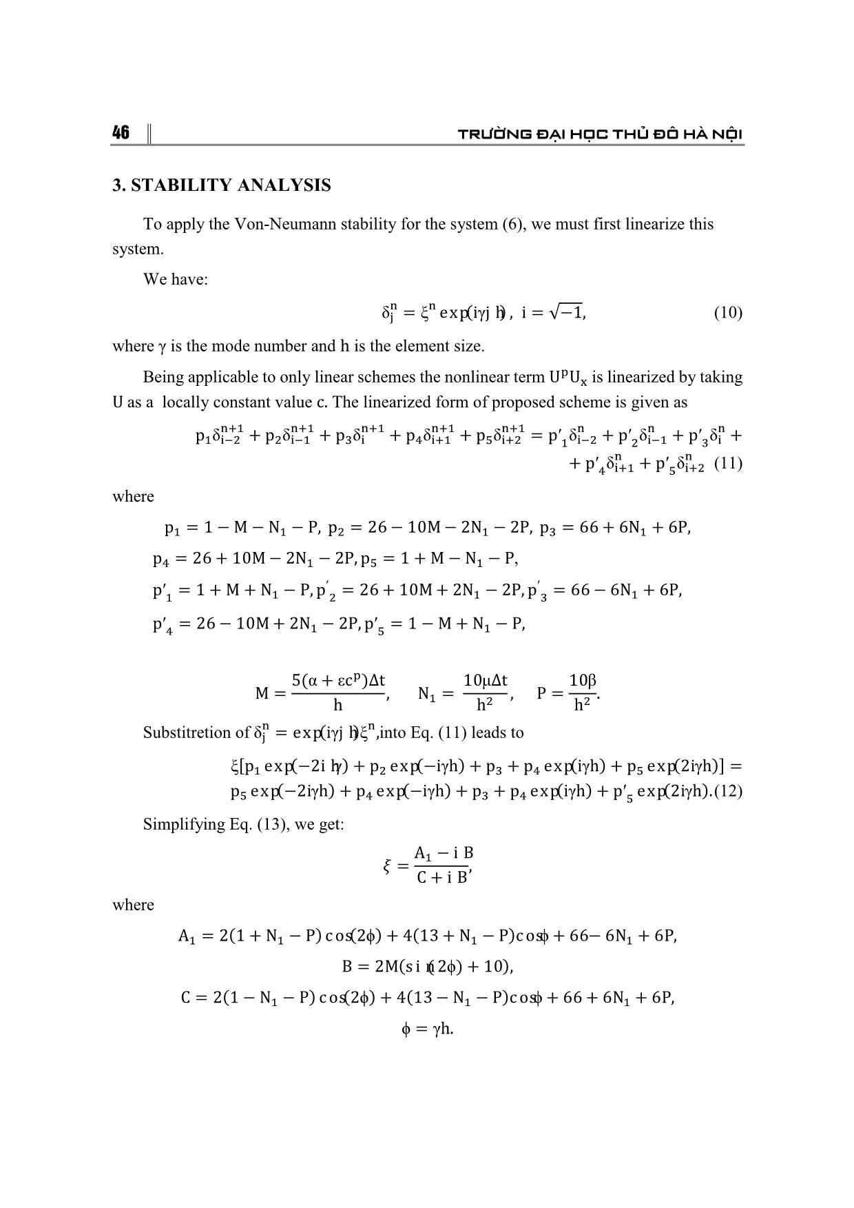
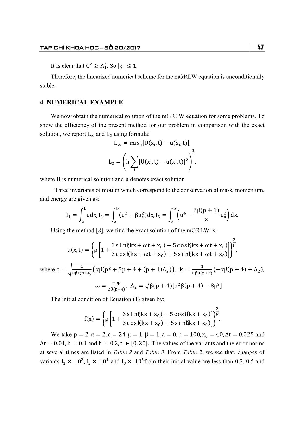
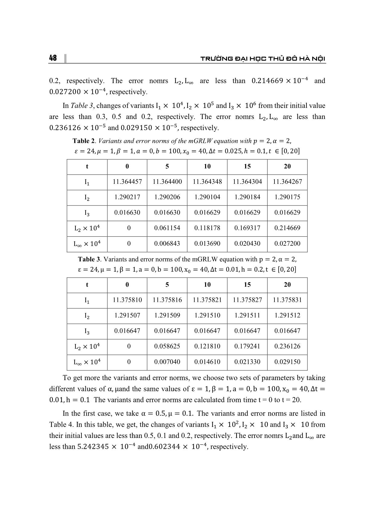
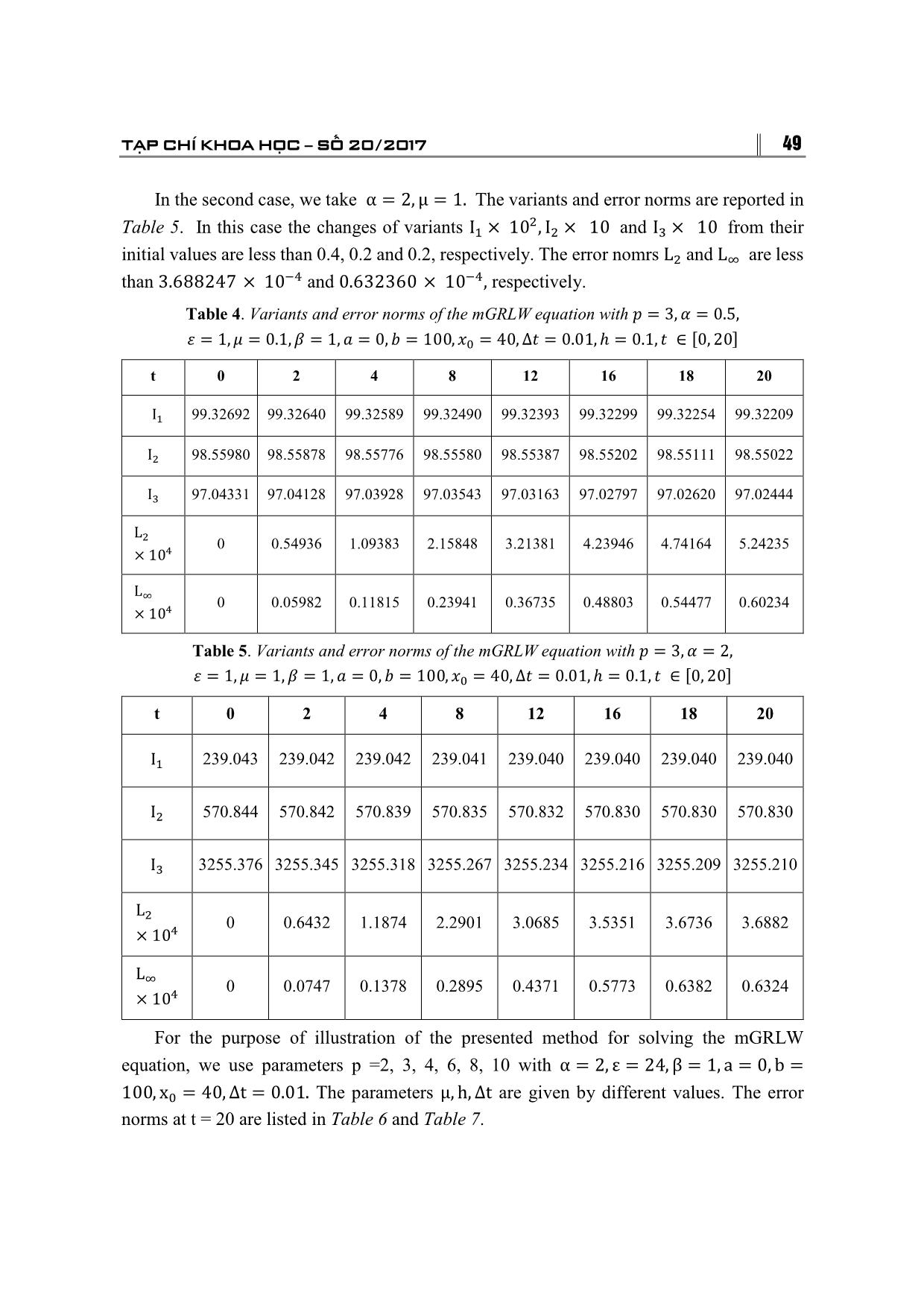
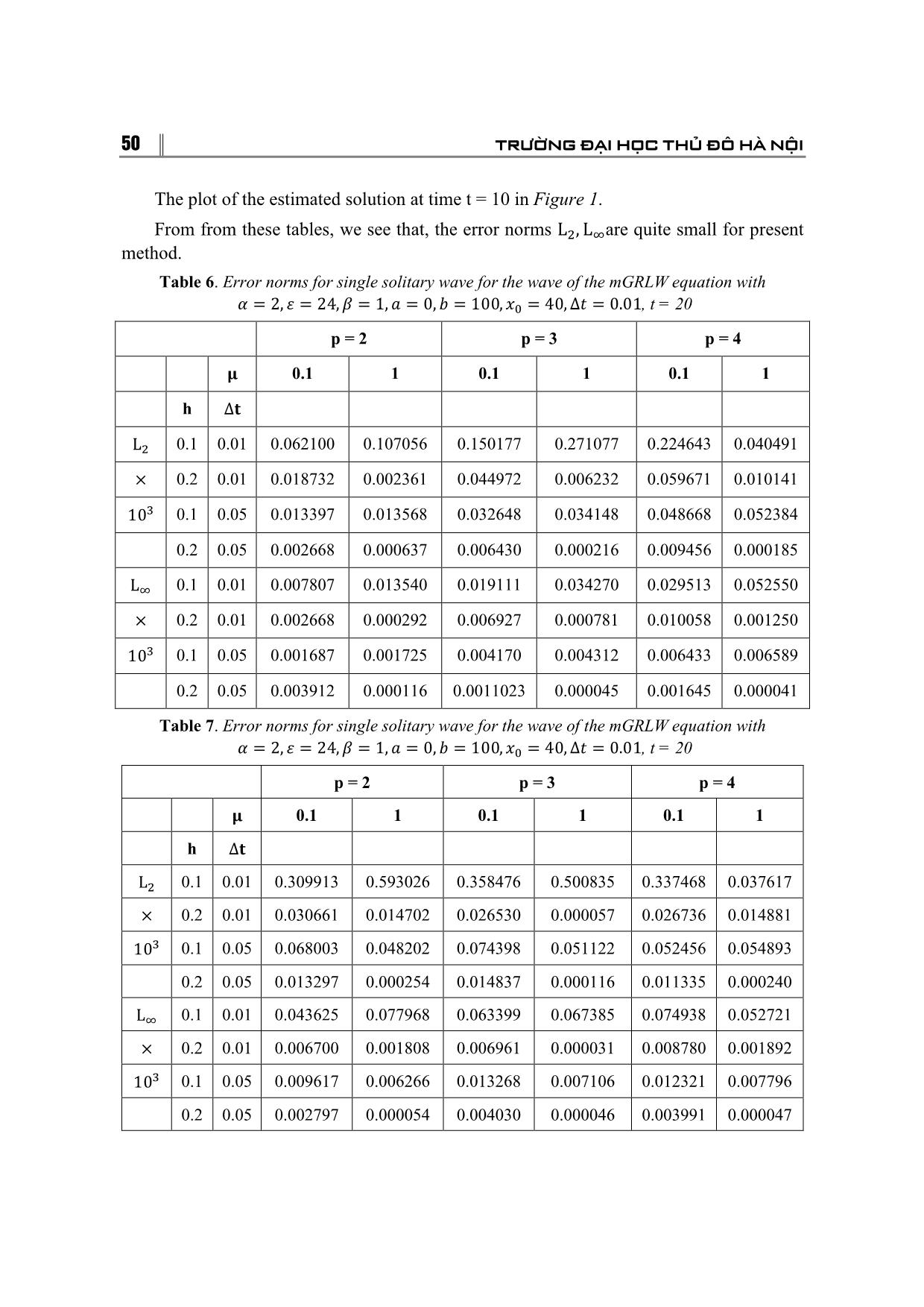
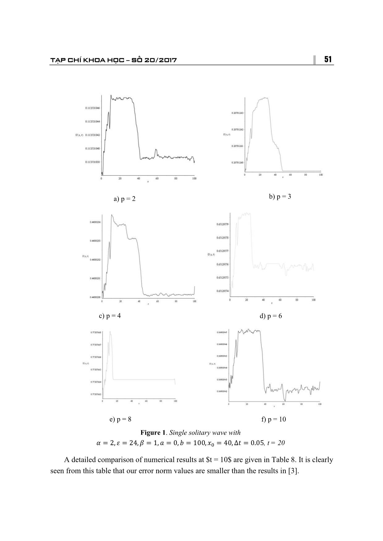
= (δ�, δ�, , δ�) , r = (f(x�), f(x�), , f(x�)) . 46 TRƯỜNG ĐẠI HỌC THỦ ĐÔ HÀ NỘI 3. STABILITY ANALYSIS To apply the Von-Neumann stability for the system (6), we must first linearize this system. We have: � � δ� = ξ exp(iγjh) , i = √−1, (10) where γ is the mode number and h is the element size. � Being applicable to only linear schemes the nonlinear term U U� is linearized by taking U as a locally constant value c. The linearized form of proposed scheme is given as ��� ��� ��� ��� ��� � � � p�δ��� + p�δ��� + p�δ� + p�δ��� + p�δ��� = p′�δ��� + p′�δ��� + p′�δ� + � � + p′�δ��� + p′�δ��� (11) where p� = 1 − M − N� − P, p� = 26 − 10M − 2N� − 2P, p� = 66 + 6N� + 6P, p� = 26 + 10M − 2N� − 2P, p� = 1 + M − N� − P, ′ ′ p′� = 1 + M + N� − P, p � = 26 + 10M + 2N� − 2P, p � = 66 − 6N� + 6P, p′� = 26 − 10M + 2N� − 2P, p′� = 1 − M + N� − P, 5(α + εc�)∆t 10μ∆t 10β M = , N = , P = . h � h� h� � � Substitretion of δ� = exp(iγjh)ξ ,into Eq. (11) leads to ξ[p� exp(−2ihγ) + p� exp(−iγh) + p� + p� exp(iγh) + p� exp(2iγh)] = p� exp(−2iγh) + p� exp(−iγh) + p� + p� exp(iγh) + p′� exp(2iγh). (12) Simplifying Eq. (13), we get: A − iB � = � , C + iB where A� = 2(1 + N� − P) cos(2ϕ) + 4(13 + N� − P)cosϕ + 66− 6N� + 6P, B = 2M(sin( 2ϕ) + 10), C = 2(1 − N� − P) cos(2ϕ) + 4(13 − N� − P)cosϕ + 66 + 6N� + 6P, ϕ = γh. TẠP CHÍ KHOA HỌC SỐ 20/2017 47 � � It is clear that C ≥ A�. So |�| ≤ 1. Therefore, the linearized numerical scheme for the mGRLW equation is unconditionally stable. 4. NUMERICAL EXAMPLE We now obtain the numerical solution of the mGRLW equation for some problems. To show the efficiency of the present method for our problem in comparison with the exact solution, we report L∞ and L� using formula: L� = max�|U(x�, t) − u(x�, t)|, � � � L� = �h �|U(x�, t) − u(x�, t)| � , � where U is numerical solution and u denotes exact solution. Three invariants of motion which correspond to the conservation of mass, momentum, and energy are given as: � � � � � � 2β(p + 1) � I� = � udx, I� = � (u + βu�)dx, I� = � �u − u�� dx. � � � ε Using the method [8], we find the exact solution of the mGRLW is: � 3 sinh(kx + ωt + x ) + 5 cosh(kx + ωt + x ) � u(x, t) = �ρ �1 + � � �� , 3 cosh(kx + ωt + x�) + 5 sinh(kx + ωt + x�) � � where ρ = � �αβ(p� + 5p + 4 + (p + 1)A )�, k = (−αβ(p + 4) + A ), ���(���) � ���(���) � ��� ω = , A = �β(p + 4)[α�β(p + 4) − 8μ�]. ��(���) � The initial condition of Equation (1) given by: � 3 sinh(kx + x ) + 5 cosh(kx + x ) � f(x) = �ρ �1 + � � �� . 3 cosh(kx + x�) + 5 sinh(kx + x�) We take p = 2, α = 2, ε = 24, μ = 1, β = 1, a = 0, b = 100, x� = 40, ∆t = 0.025 and ∆t = 0.01, h = 0.1 and h = 0.2, t ∈ [0, 20]. The values of the variants and the error norms at several times are listed in Table 2 and Table 3. From Table 2, we see that, changes of � � � variants I� × 10 , I� × 10 and I� × 10 from their initial value are less than 0.2, 0.5 and 48 TRƯỜNG ĐẠI HỌC THỦ ĐÔ HÀ NỘI �� 0.2, respectively. The error nomrs L�, L� are less than 0.214669 × 10 and 0.027200 × 10��, respectively. � � � In Table 3, changes of variants I� × 10 , I� × 10 and I� × 10 from their initial value are less than 0.3, 0.5 and 0.2, respectively. The error nomrs L�, L� are less than 0.236126 × 10�� and 0.029150 × 10��, respectively. Table 2. Variants and error norms of the mGRLW equation with � = 2, � = 2, � = 24, � = 1, � = 1, � = 0, � = 100, �� = 40, ∆� = 0.025, ℎ = 0.1, � ∈ [0, 20] t 0 5 10 15 20 I� 11.364457 11.364400 11.364348 11.364304 11.364267 I� 1.290217 1.290206 1.290104 1.290184 1.290175 I� 0.016630 0.016630 0.016629 0.016629 0.016629 � L� × 10 0 0.061154 0.118178 0.169317 0.214669 � L� × 10 0 0.006843 0.013690 0.020430 0.027200 Table 3. Variants and error norms of the mGRLW equation with p = 2, α = 2, ε = 24, μ = 1, β = 1, a = 0, b = 100, x� = 40, ∆t = 0.01, h = 0.2, t ∈ [0, 20] t 0 5 10 15 20 I� 11.375810 11.375816 11.375821 11.375827 11.375831 I� 1.291507 1.291509 1.291510 1.291511 1.291512 I� 0.016647 0.016647 0.016647 0.016647 0.016647 � L� × 10 0 0.058625 0.121810 0.179241 0.236126 � L� × 10 0 0.007040 0.014610 0.021330 0.029150 To get more the variants and error norms, we choose two sets of parameters by taking different values of α, μand the same values of ε = 1, β = 1, a = 0, b = 100, x� = 40, ∆t = 0.01, h = 0.1 The variants and error norms are calculated from time t = 0 to t = 20. In the first case, we take α = 0.5, μ = 0.1. The variants and error norms are listed in � Table 4. In this table, we get, the changes of variants I� × 10 , I� × 10 and I� × 10 from their initial values are less than 0.5, 0.1 and 0.2, respectively. The error nomrs L�and L� are less than 5.242345 × 10�� and0.602344 × 10��, respectively. TẠP CHÍ KHOA HỌC SỐ 20/2017 49 In the second case, we take α = 2, μ = 1. The variants and error norms are reported in � Table 5. In this case the changes of variants I� × 10 , I� × 10 and I� × 10 from their initial values are less than 0.4, 0.2 and 0.2, respectively. The error nomrs L� and L� are less than 3.688247 × 10�� and 0.632360 × 10��, respectively. Table 4. Variants and error norms of the mGRLW equation with � = 3, � = 0.5, � = 1, � = 0.1, � = 1, � = 0, � = 100, �� = 40, ∆� = 0.01, ℎ = 0.1, � ∈ [0, 20] t 0 2 4 8 12 16 18 20 I� 99.32692 99.32640 99.32589 99.32490 99.32393 99.32299 99.32254 99.32209 I� 98.55980 98.55878 98.55776 98.55580 98.55387 98.55202 98.55111 98.55022 I� 97.04331 97.04128 97.03928 97.03543 97.03163 97.02797 97.02620 97.02444 L � 0 0.54936 1.09383 2.15848 3.21381 4.23946 4.74164 5.24235 × 10� L � 0 0.05982 0.11815 0.23941 0.36735 0.48803 0.54477 0.60234 × 10� Table 5. Variants and error norms of the mGRLW equation with � = 3, � = 2, � = 1, � = 1, � = 1, � = 0, � = 100, �� = 40, ∆� = 0.01, ℎ = 0.1, � ∈ [0, 20] t 0 2 4 8 12 16 18 20 I� 239.043 239.042 239.042 239.041 239.040 239.040 239.040 239.040 I� 570.844 570.842 570.839 570.835 570.832 570.830 570.830 570.830 I� 3255.376 3255.345 3255.318 3255.267 3255.234 3255.216 3255.209 3255.210 L � 0 0.6432 1.1874 2.2901 3.0685 3.5351 3.6736 3.6882 × 10� L � 0 0.0747 0.1378 0.2895 0.4371 0.5773 0.6382 0.6324 × 10� For the purpose of illustration of the presented method for solving the mGRLW equation, we use parameters p =2, 3, 4, 6, 8, 10 with α = 2, ε = 24, β = 1, a = 0, b = 100, x� = 40, ∆t = 0.01. The parameters μ, h, ∆t are given by different values. The error norms at t = 20 are listed in Table 6 and Table 7. 50 TRƯỜNG ĐẠI HỌC THỦ ĐÔ HÀ NỘI The plot of the estimated solution at time t = 10 in Figure 1. From from these tables, we see that, the error norms L�, L�are quite small for present method. Table 6. Error norms for single solitary wave for the wave of the mGRLW equation with � = 2, � = 24, � = 1, � = 0, � = 100, �� = 40, ∆� = 0.01, t = 20 p = 2 p = 3 p = 4 � 0.1 1 0.1 1 0.1 1 h ∆� L� 0.1 0.01 0.062100 0.107056 0.150177 0.271077 0.224643 0.040491 × 0.2 0.01 0.018732 0.002361 0.044972 0.006232 0.059671 0.010141 10� 0.1 0.05 0.013397 0.013568 0.032648 0.034148 0.048668 0.052384 0.2 0.05 0.002668 0.000637 0.006430 0.000216 0.009456 0.000185 L� 0.1 0.01 0.007807 0.013540 0.019111 0.034270 0.029513 0.052550 × 0.2 0.01 0.002668 0.000292 0.006927 0.000781 0.010058 0.001250 10� 0.1 0.05 0.001687 0.001725 0.004170 0.004312 0.006433 0.006589 0.2 0.05 0.003912 0.000116 0.0011023 0.000045 0.001645 0.000041 Table 7. Error norms for single solitary wave for the wave of the mGRLW equation with � = 2, � = 24, � = 1, � = 0, � = 100, �� = 40, ∆� = 0.01, t = 20 p = 2 p = 3 p = 4 � 0.1 1 0.1 1 0.1 1 h ∆� L� 0.1 0.01 0.309913 0.593026 0.358476 0.500835 0.337468 0.037617 × 0.2 0.01 0.030661 0.014702 0.026530 0.000057 0.026736 0.014881 10� 0.1 0.05 0.068003 0.048202 0.074398 0.051122 0.052456 0.054893 0.2 0.05 0.013297 0.000254 0.014837 0.000116 0.011335 0.000240 L� 0.1 0.01 0.043625 0.077968 0.063399 0.067385 0.074938 0.052721 × 0.2 0.01 0.006700 0.001808 0.006961 0.000031 0.008780 0.001892 10� 0.1 0.05 0.009617 0.006266 0.013268 0.007106 0.012321 0.007796 0.2 0.05 0.002797 0.000054 0.004030 0.000046 0.003991 0.000047 TẠP CHÍ KHOA HỌC SỐ 20/2017 51 a) p = 2 b) p = 3 c) p = 4 d) p = 6 e) p = 8 f) p = 10 Figure 1. Single solitary wave with � = 2, � = 24, � = 1, � = 0, � = 100, �� = 40, ∆� = 0.05, t = 20 A detailed comparison of numerical results at $t = 10$ are given in Table 8. It is clearly seen from this table that our error norm values are smaller than the results in [3]. 52 TRƯỜNG ĐẠI HỌC THỦ ĐÔ HÀ NỘI Table 8. Error norms for single solitary wave for the wave of the mGRLW equation with � = 1, � = 1, � = 1, � = 0.5, � = 0, � = 1, �� = 30, ∆� = 0.1, t = 10 p = 2 p = 4 p = 8 Methods LIAS Our BCS LIAS Our BCS LIAS Our BCS h L� 0.25 63.77969 0.00023 63.16492 0.000008 11.50448 0.00007 × 0.125 15.82597 0.00084 15.68213 0.00008 2.98155 0.00113 10� 0.0625 3.92074 0.00141 3.88572 0.00182 0.74262 0.00075 0.03125 0.95011 0.01380 94.16614 0.00140 0.18014 0.00788 L� 0.25 93.52639 0.00042 92.62624 0.000007 18.22979 0.00010 × 0.125 23.14686 0.00212 22.94480 0.00010 4.67495 0.00200 10� 0.0625 5.89364 0.00218 5.82816 0.00290 1.16764 0.00140 0.03125 1.42826 0.01922 1.41245 0.00165 0.28796 0.01126 5. CONCLUSION In this work, we have used the quintic B - spline collocation method for solution of the mGRLW equation. We tasted our scheme through single solitary wave and the obtained results are tabulaces. These tables show that, the changes of variants are quite small. The error norms L�, L� for the inviscid and mGRLW equation are better than the ones in previous methods. So the present method is more capable for solving these equations. REFERENCES 1. S.S.Askar and A.A.Karawia (2015), “On solving pentadiagonal linear systems via transformations”, Mathematical Problems in Engineering, Vol. 2015, pp.1-9. 2. S.Battal Gazi Karakoça, Halil Zeybek (2016), “Solitary - wave solutions of the GRLW equation using septic B - spline collocation method”, Applied Mathematics and Computation, Vol. 289, pp.159-171. 3. H.Che, X.Pan, L.Zhang and Y.Wang (2012), “Numerical analysis of a linear - implicit average scheme for generalized Benjamin - Bona - Mahony - Burgers equation”, J. Applied Mathematics, Vol. 2012, pp.1-14. TẠP CHÍ KHOA HỌC SỐ 20/2017 53 4. D.J.Evans and K.R.Raslan (2005), “Solitary waves for the generalized equal width (GEW) equation”, International J. of Computer Mathematics, Vol. 82(4), pp.445-455. 5. C.M.García - Lospez, J.I.Ramos (2012), “Effects of convection on a modified GRLW equation”, Applied Mathematics and Computation, Vol. 219, pp.4118-4132. 6. C.M.García - Lospez, J.I.Ramos (2015), “Solitari waves generated by bell - shaped initial conditions in the invicis and viscous GRLW equations”, Applied Mathematical Modelling, Vol. 39 (21), pp.6645-6668. 7. P.A.Hammad, M.S.EI – Azab (2015), “A 2N order compact finite difference method for solving the generalized regularized long wave (GRLW) equation”, Applied Mathematics and Computation, Vol. 253, pp.248-261. 8. B.Hong, D.Lu (2008), “New exact solutions for the generalized BBM and Burgers - BBM equations”, World Journal of Modelling and Simulation, Vol. 4(4), pp.243-249. 9. S.Islam, F.Haq and I.A.Tirmizi (2010), “Collocation method using quartic B-spline for numerical solution of the modified equal width wave equation”, J. Appl. Math. Inform., Vol. 28(3 - 4), pp.611-624. 10. A.G.Kaplan, Y.Dereli (2017), “Numerical solutions of the GEW equation using MLS collocation method”, International Journal of Modern Physics C, Vol. 28(1), 1750011, pp.1-23. 11. M.Mohammadi, R.Mokhtari (2011), “Solving the generalized regularized long wave equation on the basis of a reproducing kernel space”, J. of Computation and Applied Mathematics, Vol. 235, pp.4003-4014. 12. R.Mokhtari, M.Mohammadi (2010), “Numerical solution of GRLW equation using sinc - collocation method”, Computer Physics Communications, Vol. 181, pp.1266-1274. 13. E.Pindza and E.Maré (2014), “Solving the generalized regularized long wave equation using a distributed approximating functional method”, International Journal of Computational Mathematics, Vol. 2014, pp.1-12. 14. P.M.Prenter (1975), “Splines and Variational Methods”, Wiley, New York. 15. T.Roshan (2011), “A Petrov – Galerkin method for solving the generalized equal width (GEW) equation”, J. Comput. Appl. Math., Vol. 235, pp.1641-1652. 16. T.Roshan (2012), “A Petrov – Galerkin method for solving the generalized regularized long wave (GRLW) equation”, Computers and Mathematics with Applications, Vol. 63, pp.943-956. 17. M.Zarebnia and R.Parvaz (2013), “Cubic B-spline collocation method for numerical solution of the Benjamin - Bona - Mahony - Burgers equation”, International Journal of Mathematical, Computational, Physical, Electrical and Computer Engineering, Vol. 7 (3), pp.540-543. 18. H.Zeybek and S.Battal Gazi Karakoça (2017), “Application of the collocation method with B - spline to the GEW equation”, Electronic Transactions on Numerical Analysis, Vol. 46, pp.71-88. 19. L.Zhang (2005), “A finite difference scheme for generalized regularized long wave equation”, Applied Mathematics and Computation, Vol. 168, pp.962-972. 20. J.Wang, F.Bai and Y.Cheng (2011), “A meshless method for the nonlinear generalized regularized long wave equation”, Chin. Phys. B, Vol. 20(3), 030206, pp.1-8. 54 TRƯỜNG ĐẠI HỌC THỦ ĐÔ HÀ NỘI PHƯƠNG PHÁP MỚI GIẢI PHƯƠNG TRÌNH MGRLW SỬ DỤNG CƠ SỞ B – SPLINE BẬC 5 Tóm tắt: Trong bài báo này, nghiệm số của phương trình mGRLW sẽ tìm được dựa trên cơ sở phương pháp mới sử dụng cơ sở B – spline bậc 5. Sử dụng phương pháp Von – Neumann hệ phương trình sai phân ổn định vô điều kiện. Thuật toán được với sóng đơn được áp dụng giải một số ví dụ. Kết quả số chứng tỏ phương pháp đưa ra hữu hiệu để giải phương trình trên. Từ khóa: Phương trình mGRLW, spline bậc 5, phương pháp collocation, phương pháp sai phân hữu hạn.
File đính kèm:
 a_new_method_for_solving_the_mgrlw_equation_using_a_base_of.pdf

