Estimation of shale volume from well logging data using Artificial Neural Network
The existence of shale has a major effect on reservoir quality because it
reduces the rock’s both the porosity and permeability. There are several
types of shale, and they can be distributed in the sand in four different
ways: laminated, structural, dispersed, or any combination of these. Each
of them has various features and physical properties. Therefore, shale
volume estimation is one of the most important and challengin tasks to be
solved information evaluation. There are many equations proposed to
calculate shale volume from Gamma - ray log; however, none of them
could be considered the best method that can be applied to all case studies.
This study aims to propose a new approach to estimate shale volume from
well - logging data. Gamma - ray and other logs were used as input data
for an artificial neural network (ANN) to predict the shale volume. We
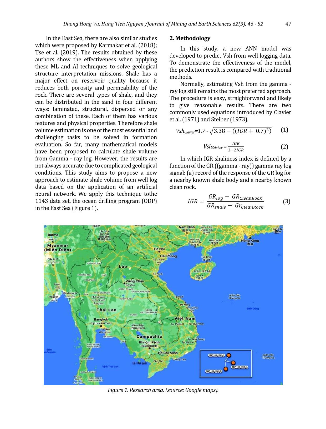
apply this technique to the 1143 data set of the ocean drilling program
(ODP) in the East Sea. The authors compared the result to core data and
recognized that utilization of several logs and ANN gives a better
estimation than conventional methods (more accurate and can reflect the
trend of actual shale volume).
Trang 1
Trang 2
Trang 3
Trang 4
Trang 5
Trang 6
Trang 7
Tóm tắt nội dung tài liệu: Estimation of shale volume from well logging data using Artificial Neural Network
fication. To overcome these
challenges, now computational tools such as
machine learning (ML) and artificial intelligence
(AI) are being used more and more in data
processing, including geophysical processing.
Specifically, the application of these tools for the
analysis of well log data has been published by
Saumen Maiti et al. (2007), Bosch et al. (2013),
Dekkers et al. (2014), and Aarushi Gupta and
Utkarsh Soumya (2020).
_____________________
*Corresponding author
E - mail: vuhongduong@humg.edu.vn
DOI: 10.46326/JMES.2021.62(3).06
 Duong Hong Vu, Hung Tien Nguyen /Journal of Mining and Earth Sciences 62(3), 46 - 52 47
In the East Sea, there are also similar studies
which were proposed by Karmakar et al. (2018);
Tse et al. (2019). The results obtained by these
authors show the effectiveness when applying
these ML and AI techniques to solve geological
structure interpretation missions. Shale has a
major effect on reservoir quality because it
reduces both porosity and permeability of the
rock. There are several types of shale, and they
can be distributed in the sand in four different
ways: laminated, structural, dispersed or any
combination of these. Each of them has various
features and physical properties. Therefore shale
volume estimation is one of the most essential and
challenging tasks to be solved in formation
evaluation. So far, many mathematical models
have been proposed to calculate shale volume
from Gamma - ray log. However, the results are
not always accurate due to complicated geological
conditions. This study aims to propose a new
approach to estimate shale volume from well log
data based on the application of an artificial
neural network. We apply this technique tothe
1143 data set, the ocean drilling program (ODP)
in the East Sea (Figure 1).
2. Methodology
In this study, a new ANN model was
developed to predict Vsh from well logging data.
To demonstrate the effectiveness of the model,
the prediction result is compared with traditional
methods.
Normally, estimating Vsh from the gamma -
ray log still remains the most preferred approach.
The procedure is easy, straighforward and likely
to give reasonable results. There are two
commonly used equations introduced by Clavier
et al. (1971) and Steiber (1973).
VshClavier=1.7 - √3.38 − ((𝐼𝐺𝑅 + 0.7)2) (1)
VshStieber =
𝐼𝐺𝑅
3−2𝐼𝐺𝑅
 (2)
In which IGR shaliness index is defined by a
function of the GR ((gamma - ray)) gamma ray log
signal: (a) record of the response of the GR log for
a nearby known shale body and a nearby known
clean rock.
𝐼𝐺𝑅 =
𝐺𝑅𝑙𝑜𝑔 − 𝐺𝑅𝐶𝑙𝑒𝑎𝑛𝑅𝑜𝑐𝑘
𝐺𝑅𝑠ℎ𝑎𝑙𝑒 − 𝐺𝑟𝐶𝑙𝑒𝑎𝑛𝑅𝑜𝑐𝑘
 (3)
Figure 1. Research area. (source: Google maps).
48 Duong Hong Vu, Hung Tien Nguyen /Journal of Mining and Earth Sciences 62(3), 46 - 52
An ANN network using back - propagation
training algorithm (BPNN) and logsig activation
function was proposed to predict the volume of
shale from well - logging data. We used data from
well A and B to train the ANN model, then used
data of well C to evaluate the accuracy of the
prediction model. Finally, the proposed ANN
model was used to predict Vsh from input data of
well C; then its performance was compared to
Clavier and Steiber model.
3. Data sets
In this study, we used data sources from
International Ocean Discovery Program
( At this location,
there are three wells OPD - 184 - 1143 A, B, and C
(Figure 1), for brevity in this article we named
them well A, B, C, respectively (Figure 1).
The data used in this study include physical
and lithological parameters measured in a
borehole such as the longitudinal wave velocity
(Vp), gamma - ray, density, magnetic
susceptibility, and volume of shale (Vsh) in the
core sample (Table 1).
3.1. Data preprocessing
Abnormal data can be considered as noise
because they can negatively influence the ANN
model and may restrict the model in its
generalization. The data set of three wells are
tested for anomaly by Z - score outlier detection
algorithm where a threshold Z - Score of 3 is
selected (Tripathy et al., 2013). Any data points
above this threshold are marked as an outlier and
excluded from the training data. The Z - score is
the score given to the participant as per their
performance:
z = |Xi - Xmean|/ SD (4)
Where: Xmean - the mean value of the data; SD
- the standard deviation of the data; SD - the
standard deviation of the data.
To simplify the interpretation of the z - scores,
the following agreements were made as:
z < 2 implies the result is satisfactory.
2 < z < 3 implies the result is questionable.
z > 3 implies the result is unsatisfactory.
To reduce volatility and eliminate statistical
noise, the dataset is further processed and
smoothened by a low - pass second – order
Butterworth filter (Selesnick and Burrus, 1998).
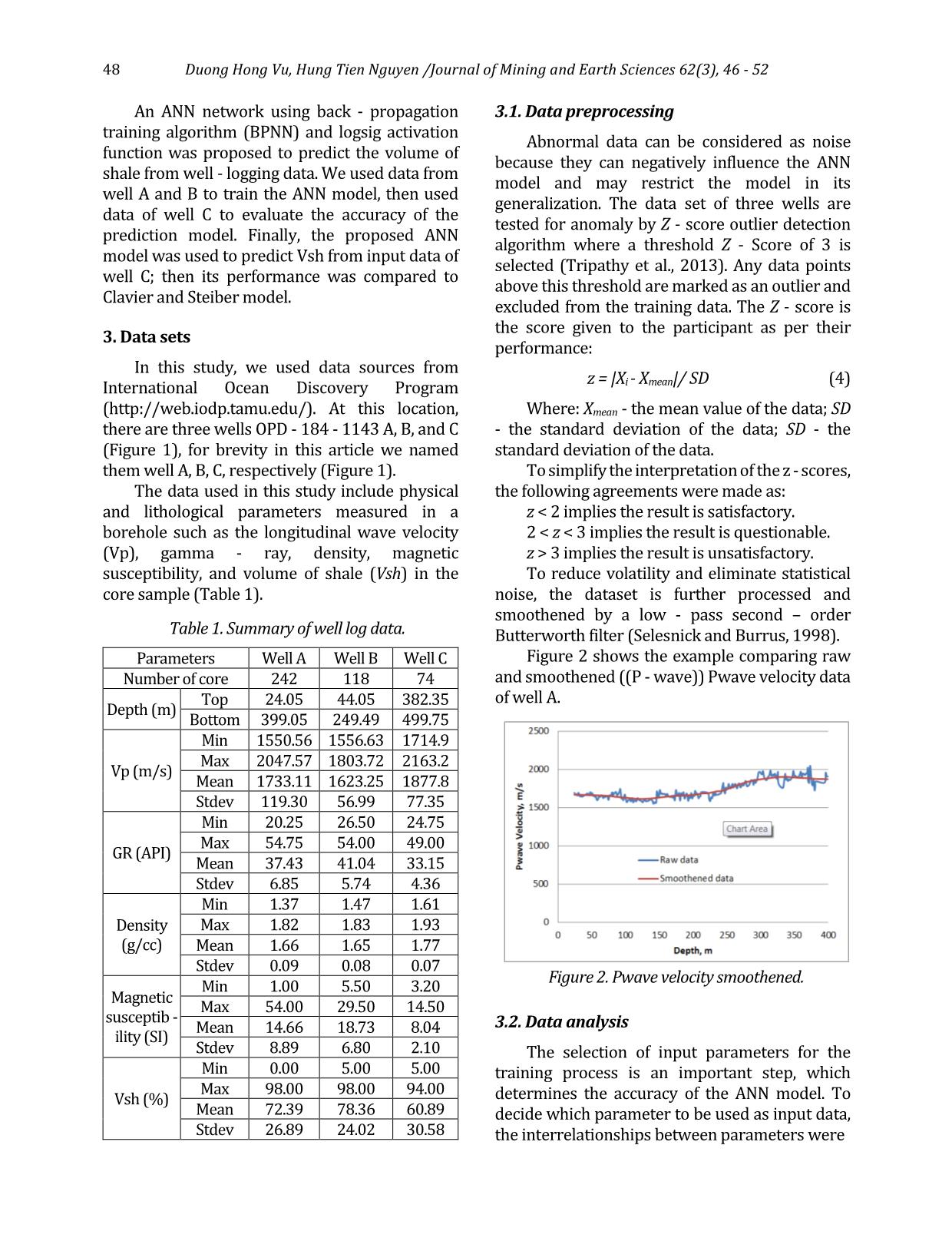
Figure 2 shows the example comparing raw
and smoothened ((P - wave)) Pwave velocity data
of well A.
3.2. Data analysis
The selection of input parameters for the
training process is an important step, which
determines the accuracy of the ANN model. To
decide which parameter to be used as input data,
the interrelationships between parameters were
Parameters Well A Well B Well C
Number of core 242 118 74
Depth (m)
Top 24.05 44.05 382.35
Bottom 399.05 249.49 499.75
Vp (m/s)
Min 1550.56 1556.63 1714.9
Max 2047.57 1803.72 2163.2
Mean 1733.11 1623.25 1877.8
Stdev 119.30 56.99 77.35
GR (API)
Min 20.25 26.50 24.75
Max 54.75 54.00 49.00
Mean 37.43 41.04 33.15
Stdev 6.85 5.74 4.36
Density
(g/cc)
Min 1.37 1.47 1.61
Max 1.82 1.83 1.93
Mean 1.66 1.65 1.77
Stdev 0.09 0.08 0.07
Magnetic
susceptib -
ility (SI)
Min 1.00 5.50 3.20
Max 54.00 29.50 14.50
Mean 14.66 18.73 8.04
Stdev 8.89 6.80 2.10
Vsh (%)
Min 0.00 5.00 5.00
Max 98.00 98.00 94.00
Mean 72.39 78.36 60.89
Stdev 26.89 24.02 30.58
Table 1. Summary of well log data.
Figure 2. Pwave velocity smoothened.
 Duong Hong Vu, Hung Tien Nguyen /Journal of Mining and Earth Sciences 62(3), 46 - 52 49
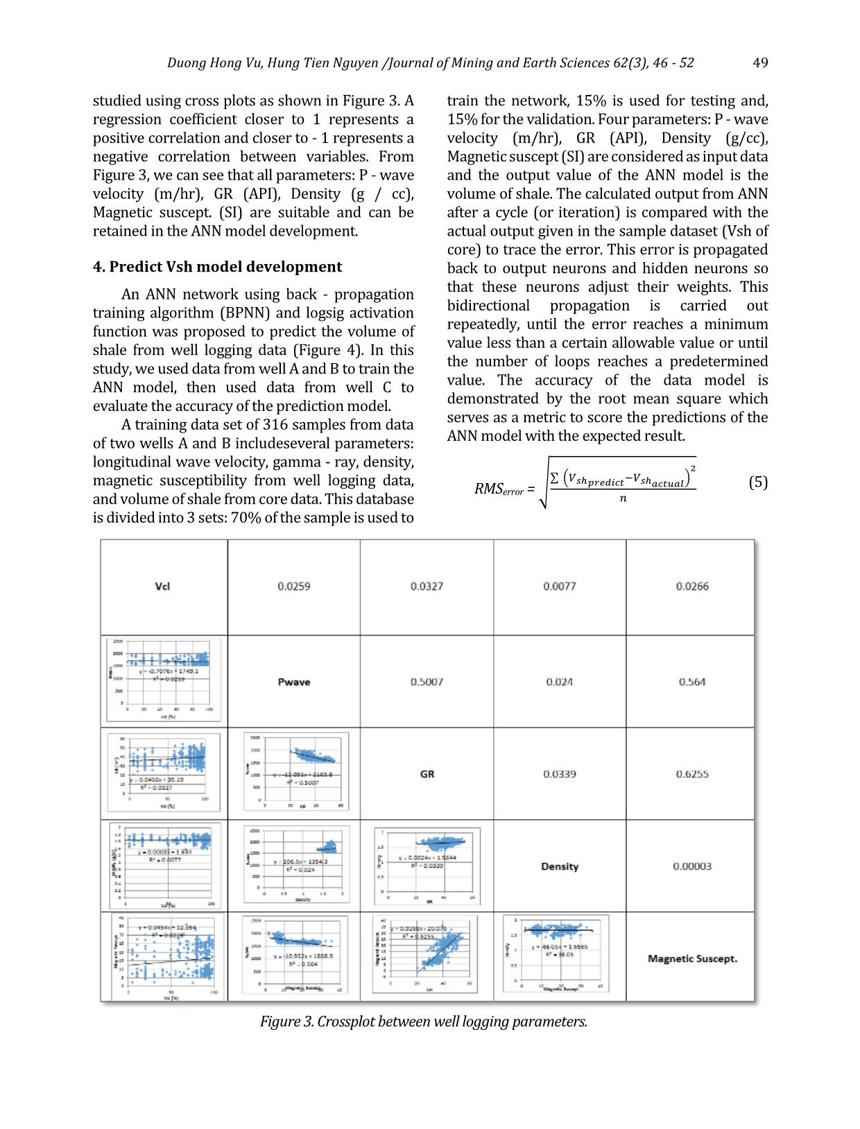
studied using cross plots as shown in Figure 3. A
regression coefficient closer to 1 represents a
positive correlation and closer to - 1 represents a
negative correlation between variables. From
Figure 3, we can see that all parameters: P - wave
velocity (m/hr), GR (API), Density (g / cc),
Magnetic suscept. (SI) are suitable and can be
retained in the ANN model development.
4. Predict Vsh model development
An ANN network using back - propagation
training algorithm (BPNN) and logsig activation
function was proposed to predict the volume of
shale from well logging data (Figure 4). In this
study, we used data from well A and B to train the
ANN model, then used data from well C to
evaluate the accuracy of the prediction model.
A training data set of 316 samples from data
of two wells A and B includeseveral parameters:
longitudinal wave velocity, gamma - ray, density,
magnetic susceptibility from well logging data,
and volume of shale from core data. This database
is divided into 3 sets: 70% of the sample is used to
train the network, 15% is used for testing and,
15% for the validation. Four parameters: P - wave
velocity (m/hr), GR (API), Density (g/cc),
Magnetic suscept (SI) are considered as input data
and the output value of the ANN model is the
volume of shale. The calculated output from ANN
after a cycle (or iteration) is compared with the
actual output given in the sample dataset (Vsh of
core) to trace the error. This error is propagated
back to output neurons and hidden neurons so
that these neurons adjust their weights. This
bidirectional propagation is carried out
repeatedly, until the error reaches a minimum
value less than a certain allowable value or until
the number of loops reaches a predetermined
value. The accuracy of the data model is
demonstrated by the root mean square which
serves as a metric to score the predictions of the
ANN model with the expected result.
RMSerror = √
∑ (𝑉𝑠ℎ𝑝𝑟𝑒𝑑𝑖𝑐𝑡−𝑉𝑠ℎ𝑎𝑐𝑡𝑢𝑎𝑙)
2
𝑛
 (5)
Figure 3. Crossplot between well logging parameters.
50 Duong Hong Vu, Hung Tien Nguyen /Journal of Mining and Earth Sciences 62(3), 46 - 52
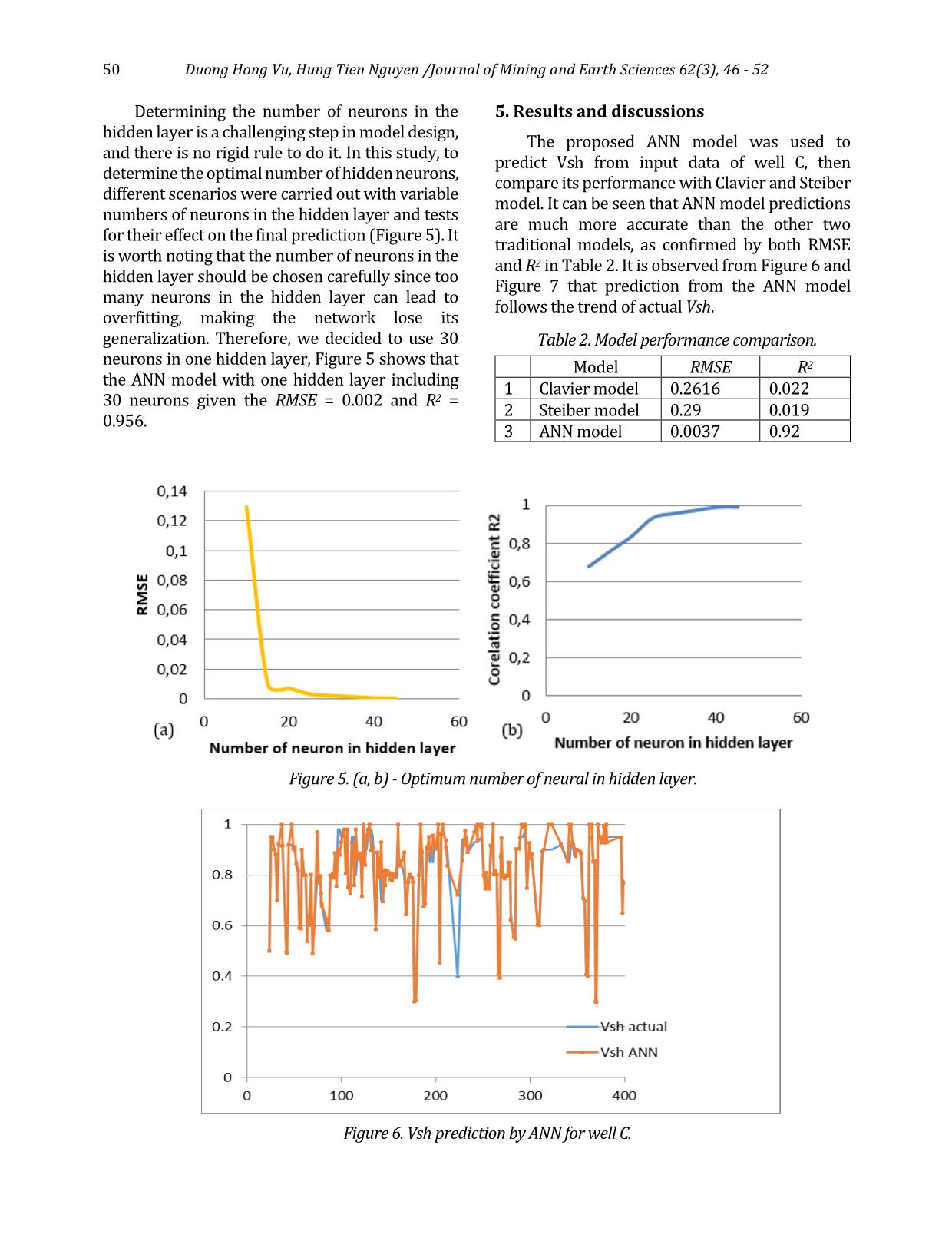
Determining the number of neurons in the
hidden layer is a challenging step in model design,
and there is no rigid rule to do it. In this study, to
determine the optimal number of hidden neurons,
different scenarios were carried out with variable
numbers of neurons in the hidden layer and tests
for their effect on the final prediction (Figure 5). It
is worth noting that the number of neurons in the
hidden layer should be chosen carefully since too
many neurons in the hidden layer can lead to
overfitting, making the network lose its
generalization. Therefore, we decided to use 30
neurons in one hidden layer, Figure 5 shows that
the ANN model with one hidden layer including
30 neurons given the RMSE = 0.002 and R2 =
0.956.
5. Results and discussions
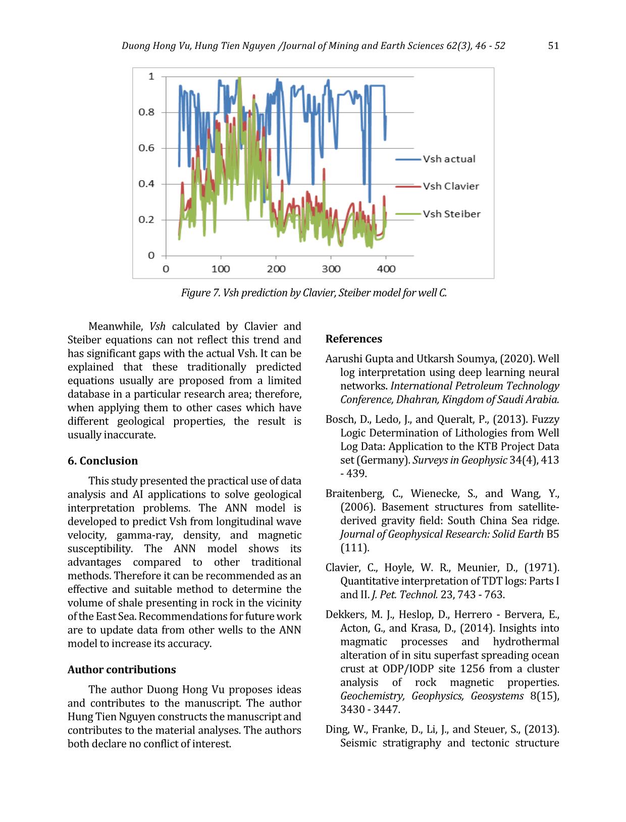
The proposed ANN model was used to
predict Vsh from input data of well C, then
compare its performance with Clavier and Steiber
model. It can be seen that ANN model predictions
are much more accurate than the other two
traditional models, as confirmed by both RMSE
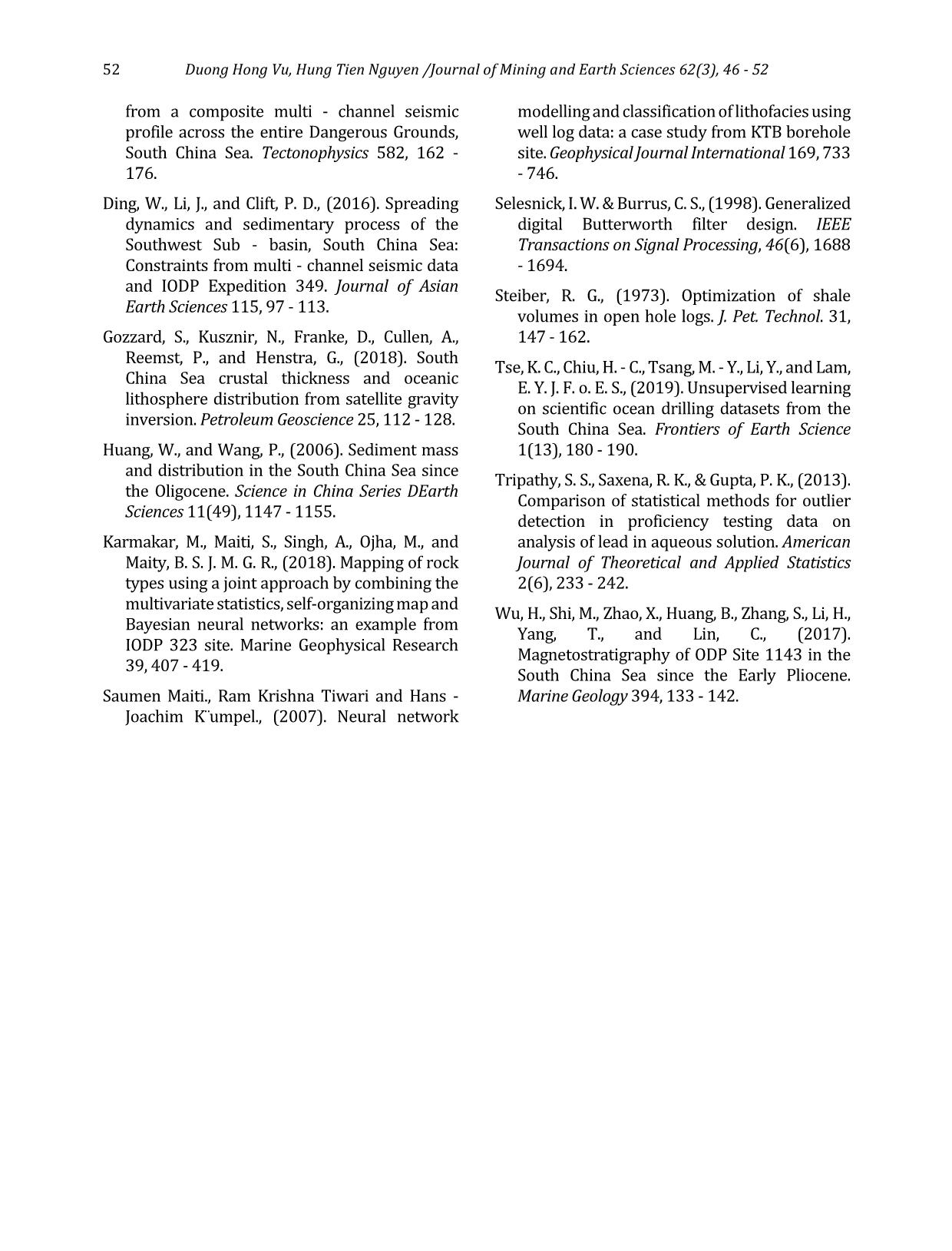
and R2 in Table 2. It is observed from Figure 6 and
Figure 7 that prediction from the ANN model
follows the trend of actual Vsh.
 Model RMSE R2
1 Clavier model 0.2616 0.022
2 Steiber model 0.29 0.019
3 ANN model 0.0037 0.92
Table 2. Model performance comparison.
Figure 5. (a, b) - Optimum number of neural in hidden layer.
Figure 6. Vsh prediction by ANN for well C.
 Duong Hong Vu, Hung Tien Nguyen /Journal of Mining and Earth Sciences 62(3), 46 - 52 51
Meanwhile, Vsh calculated by Clavier and
Steiber equations can not reflect this trend and
has significant gaps with the actual Vsh. It can be
explained that these traditionally predicted
equations usually are proposed from a limited
database in a particular research area; therefore,
when applying them to other cases which have
different geological properties, the result is
usually inaccurate.
6. Conclusion
This study presented the practical use of data
analysis and AI applications to solve geological
interpretation problems. The ANN model is
developed to predict Vsh from longitudinal wave
velocity, gamma-ray, density, and magnetic
susceptibility. The ANN model shows its
advantages compared to other traditional
methods. Therefore it can be recommended as an
effective and suitable method to determine the
volume of shale presenting in rock in the vicinity
of the East Sea. Recommendations for future work
are to update data from other wells to the ANN
model to increase its accuracy.
Author contributions
The author Duong Hong Vu proposes ideas
and contributes to the manuscript. The author
Hung Tien Nguyen constructs the manuscript and
contributes to the material analyses. The authors
both declare no conflict of interest.
References
Aarushi Gupta and Utkarsh Soumya, (2020). Well
log interpretation using deep learning neural
networks. International Petroleum Technology
Conference, Dhahran, Kingdom of Saudi Arabia.
Bosch, D., Ledo, J., and Queralt, P., (2013). Fuzzy
Logic Determination of Lithologies from Well
Log Data: Application to the KTB Project Data
set (Germany). Surveys in Geophysic 34(4), 413
- 439.
Braitenberg, C., Wienecke, S., and Wang, Y.,
(2006). Basement structures from satellite-
derived gravity field: South China Sea ridge.
Journal of Geophysical Research: Solid Earth B5
(111).
Clavier, C., Hoyle, W. R., Meunier, D., (1971).
Quantitative interpretation of TDT logs: Parts I
and II. J. Pet. Technol. 23, 743 - 763.
Dekkers, M. J., Heslop, D., Herrero - Bervera, E.,
Acton, G., and Krasa, D., (2014). Insights into
magmatic processes and hydrothermal
alteration of in situ superfast spreading ocean
crust at ODP/IODP site 1256 from a cluster
analysis of rock magnetic properties.
Geochemistry, Geophysics, Geosystems 8(15),
3430 - 3447.
Ding, W., Franke, D., Li, J., and Steuer, S., (2013).
Seismic stratigraphy and tectonic structure
Figure 7. Vsh prediction by Clavier, Steiber model for well C.
52 Duong Hong Vu, Hung Tien Nguyen /Journal of Mining and Earth Sciences 62(3), 46 - 52
from a composite multi - channel seismic
profile across the entire Dangerous Grounds,
South China Sea. Tectonophysics 582, 162 -
176.
Ding, W., Li, J., and Clift, P. D., (2016). Spreading
dynamics and sedimentary process of the
Southwest Sub - basin, South China Sea:
Constraints from multi - channel seismic data
and IODP Expedition 349. Journal of Asian
Earth Sciences 115, 97 - 113.
Gozzard, S., Kusznir, N., Franke, D., Cullen, A.,
Reemst, P., and Henstra, G., (2018). South
China Sea crustal thickness and oceanic
lithosphere distribution from satellite gravity
inversion. Petroleum Geoscience 25, 112 - 128.
Huang, W., and Wang, P., (2006). Sediment mass
and distribution in the South China Sea since
the Oligocene. Science in China Series DEarth
Sciences 11(49), 1147 - 1155.
Karmakar, M., Maiti, S., Singh, A., Ojha, M., and
Maity, B. S. J. M. G. R., (2018). Mapping of rock
types using a joint approach by combining the
multivariate statistics, self-organizing map and
Bayesian neural networks: an example from
IODP 323 site. Marine Geophysical Research
39, 407 - 419.
Saumen Maiti., Ram Krishna Tiwari and Hans -
Joachim K¨umpel., (2007). Neural network
modelling and classification of lithofacies using
well log data: a case study from KTB borehole
site. Geophysical Journal International 169, 733
- 746.
Selesnick, I. W. & Burrus, C. S., (1998). Generalized
digital Butterworth filter design. IEEE
Transactions on Signal Processing, 46(6), 1688
- 1694.
Steiber, R. G., (1973). Optimization of shale
volumes in open hole logs. J. Pet. Technol. 31,
147 - 162.
Tse, K. C., Chiu, H. - C., Tsang, M. - Y., Li, Y., and Lam,
E. Y. J. F. o. E. S., (2019). Unsupervised learning
on scientific ocean drilling datasets from the
South China Sea. Frontiers of Earth Science
1(13), 180 - 190.
Tripathy, S. S., Saxena, R. K., & Gupta, P. K., (2013).
Comparison of statistical methods for outlier
detection in proficiency testing data on
analysis of lead in aqueous solution. American
Journal of Theoretical and Applied Statistics
2(6), 233 - 242.
Wu, H., Shi, M., Zhao, X., Huang, B., Zhang, S., Li, H.,
Yang, T., and Lin, C., (2017).
Magnetostratigraphy of ODP Site 1143 in the
South China Sea since the Early Pliocene.
Marine Geology 394, 133 - 142.
File đính kèm:
 estimation_of_shale_volume_from_well_logging_data_using_arti.pdf

