Efficient market hypothesis and calendar effects: Empirical evidences from the Vietnam stock markets

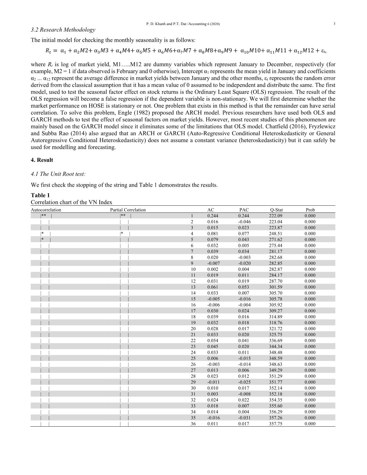
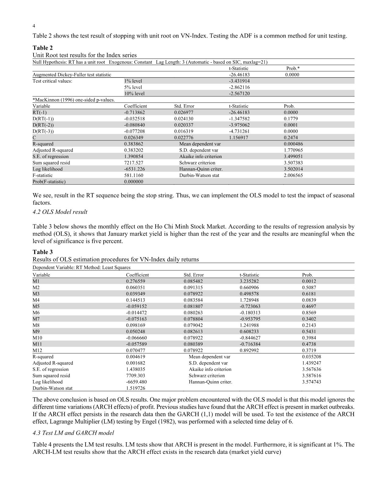
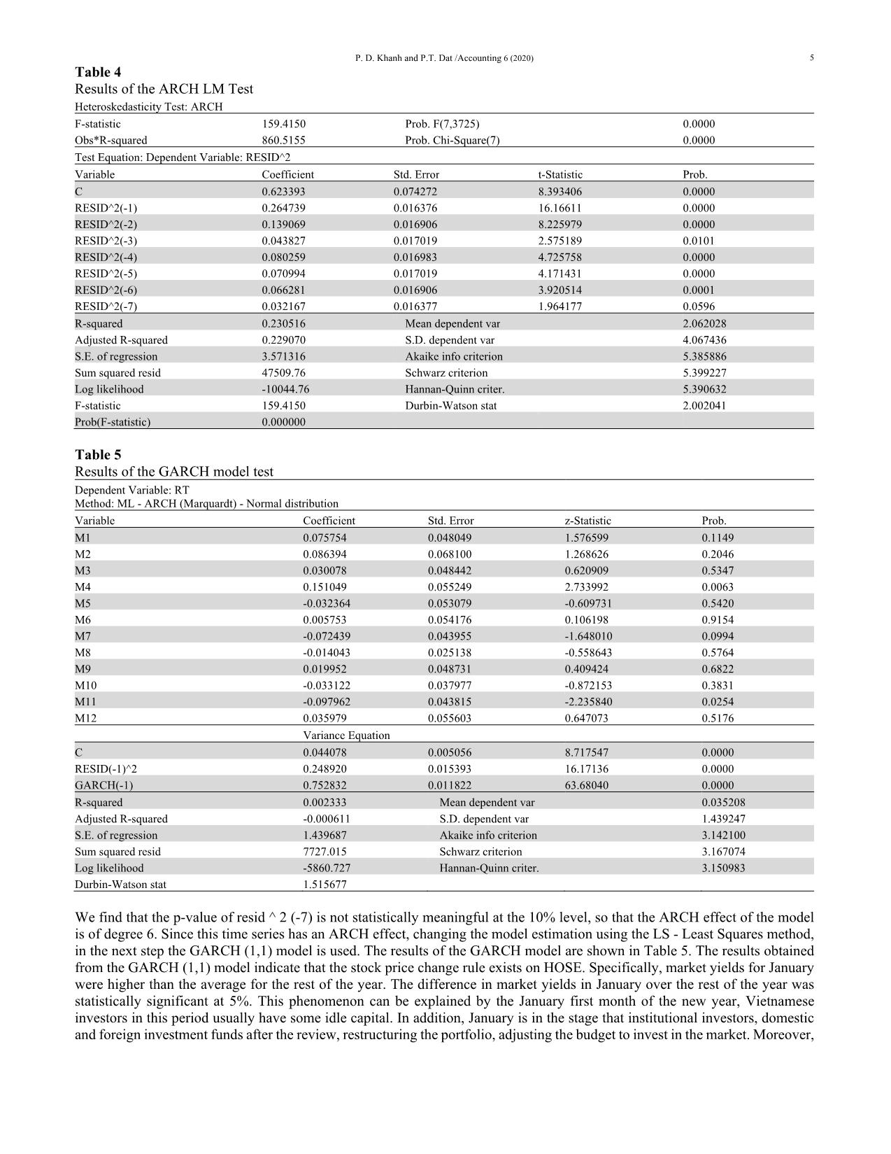
as follows: 
𝑅௧ = αଵ + αଶ𝑀2+ αଷ𝑀3 + αସ𝑀4+ αହ𝑀5 + α଺𝑀6+α଻𝑀7 + α଼𝑀8+αଽ𝑀9 + αଵ଴𝑀10+ αଵଵ𝑀11 + αଵଶ𝑀12 + εt, 
where Rt is log of market yield, M1..M12 are dummy variables which represent January to December, respectively (for 
example, M2 = 1 if data observed is February and 0 otherwise), Intercept α1 represents the mean yield in January and coefficients 
α2 ... α12 represent the average difference in market yields between January and the other months, εt represents the random error 
derived from the classical assumption that it has a mean value of 0 assumed to be independent and distribute the same. The first 
model, used to test the seasonal factor effect on stock returns is the Ordinary Least Square (OLS) regression. The result of the 
OLS regression will become a false regression if the dependent variable is non-stationary. We will first determine whether the 
market performance on HOSE is stationary or not. One problem that exists in this method is that the remainder can have serial 
correlation. To solve this problem, Engle (1982) proposed the ARCH model. Previous researchers have used both OLS and 
GARCH methods to test the effect of seasonal factors on market yields. However, most recent studies of this phenomenon are 
mainly based on the GARCH model since it eliminates some of the limitations that OLS model. Chatfield (2016), Fryzlewicz 
and Subba Rao (2014) also argued that an ARCH or GARCH (Auto-Regressive Conditional Heteroskedasticity or General 
Autoregressive Conditional Heteroskedasticity) does not assume a constant variance (heteroskedasticity) but it can safely be 
used for modelling and forecasting. 
4. Result 
4.1 The Unit Root test: 
We first check the stopping of the string and Table 1 demonstrates the results. 
Table 1 
Correlation chart of the VN Index 
Autocorrelation Partial Correlation AC PAC Q-Stat Prob 
 |** | |** | 1 0.244 0.244 222.09 0.000 
 | | | | 2 0.016 -0.046 223.04 0.000 
 | | | | 3 0.015 0.023 223.87 0.000 
 |* | |* | 4 0.081 0.077 248.51 0.000 
 |* | | | 5 0.079 0.043 271.62 0.000 
 | | | | 6 0.032 0.005 275.44 0.000 
 | | | | 7 0.039 0.034 281.17 0.000 
 | | | | 8 0.020 -0.003 282.68 0.000 
 | | | | 9 -0.007 -0.020 282.85 0.000 
 | | | | 10 0.002 0.004 282.87 0.000 
 | | | | 11 0.019 0.011 284.17 0.000 
 | | | | 12 0.031 0.019 287.70 0.000 
 | | | | 13 0.061 0.053 301.59 0.000 
 | | | | 14 0.033 0.007 305.70 0.000 
 | | | | 15 -0.005 -0.016 305.78 0.000 
 | | | | 16 -0.006 -0.004 305.92 0.000 
 | | | | 17 0.030 0.024 309.27 0.000 
 | | | | 18 0.039 0.016 314.89 0.000 
 | | | | 19 0.032 0.018 318.76 0.000 
 | | | | 20 0.028 0.017 321.72 0.000 
 | | | | 21 0.033 0.020 325.75 0.000 
 | | | | 22 0.054 0.041 336.69 0.000 
 | | | | 23 0.045 0.020 344.34 0.000 
 | | | | 24 0.033 0.011 348.48 0.000 
 | | | | 25 0.006 -0.015 348.59 0.000 
 | | | | 26 -0.003 -0.014 348.63 0.000 
 | | | | 27 0.013 0.006 349.29 0.000 
 | | | | 28 0.023 0.012 351.29 0.000 
 | | | | 29 -0.011 -0.025 351.77 0.000 
 | | | | 30 0.010 0.017 352.14 0.000 
 | | | | 31 0.003 -0.008 352.18 0.000 
 | | | | 32 0.024 0.022 354.35 0.000 
 | | | | 33 0.018 0.007 355.60 0.000 
 | | | | 34 0.014 0.004 356.29 0.000 
 | | | | 35 -0.016 -0.031 357.26 0.000 
 | | | | 36 0.011 0.017 357.75 0.000 
 4
Table 2 shows the test result of stopping with unit root on VN-Index. Testing the ADF is a common method for unit testing. 
Table 2 
Unit Root test results for the Index series 
Null Hypothesis: RT has a unit root Exogenous: Constant Lag Length: 3 (Automatic - based on SIC, maxlag=21) 
 t-Statistic Prob.* 
Augmented Dickey-Fuller test statistic -26.46183 0.0000 
Test critical values: 1% level -3.431914 
 5% level -2.862116 
 10% level -2.567120 
*MacKinnon (1996) one-sided p-values. 
Variable Coefficient Std. Error t-Statistic Prob. 
RT(-1) -0.713862 0.026977 -26.46183 0.0000 
D(RT(-1)) -0.032518 0.024130 -1.347582 0.1779 
D(RT(-2)) -0.080840 0.020337 -3.975062 0.0001 
D(RT(-3)) -0.077208 0.016319 -4.731261 0.0000 
C 0.026349 0.022776 1.156917 0.2474 
R-squared 0.383862 Mean dependent var 0.000486 
Adjusted R-squared 0.383202 S.D. dependent var 1.770965 
S.E. of regression 1.390854 Akaike info criterion 3.499051 
Sum squared resid 7217.527 Schwarz criterion 3.507383 
Log likelihood -6531.226 Hannan-Quinn criter. 3.502014 
F-statistic 581.1160 Durbin-Watson stat 2.006565 
Prob(F-statistic) 0.000000 
We see, result in the RT sequence being the stop string. Thus, we can implement the OLS model to test the impact of seasonal 
factors. 
4.2 OLS Model result 
Table 3 below shows the monthly effect on the Ho Chi Minh Stock Market. According to the results of regression analysis by 
method (OLS), it shows that January market yield is higher than the rest of the year and the results are meaningful when the 
level of significance is five percent. 
Table 3 
Results of OLS estimation procedures for VN-Index daily returns 
Dependent Variable: RT Method: Least Squares 
Variable Coefficient Std. Error t-Statistic Prob. 
M1 0.276559 0.085482 3.235282 0.0012 
M2 0.060351 0.091315 0.660906 0.5087 
M3 0.039349 0.078922 0.498578 0.6181 
M4 0.144513 0.083584 1.728948 0.0839 
M5 -0.059152 0.081807 -0.723063 0.4697 
M6 -0.014472 0.080263 -0.180313 0.8569 
M7 -0.075163 0.078804 -0.953795 0.3402 
M8 0.098169 0.079042 1.241988 0.2143 
M9 0.050248 0.082613 0.608233 0.5431 
M10 -0.066660 0.078922 -0.844627 0.3984 
M11 -0.057589 0.080389 -0.716384 0.4738 
M12 0.070477 0.078922 0.892992 0.3719 
R-squared 0.004619 Mean dependent var 0.035208 
Adjusted R-squared 0.001682 S.D. dependent var 1.439247 
S.E. of regression 1.438035 Akaike info criterion 3.567636 
Sum squared resid 7709.303 Schwarz criterion 3.587616 
Log likelihood -6659.480 Hannan-Quinn criter. 3.574743 
Durbin-Watson stat 1.519726 
The above conclusion is based on OLS results. One major problem encountered with the OLS model is that this model ignores the 
different time variations (ARCH effects) of profit. Previous studies have found that the ARCH effect is present in market outbreaks. 
If the ARCH effect persists in the research data then the GARCH (1,1) model will be used. To test the existence of the ARCH 
effect, Lagrange Multiplier (LM) testing by Engel (1982), was performed with a selected time delay of 6. 
4.3 Test LM and GARCH model 
Table 4 presents the LM test results. LM tests show that ARCH is present in the model. Furthermore, it is significant at 1%. The 
ARCH-LM test results show that the ARCH effect exists in the research data (market yield curve) 
P. D. Khanh and P.T. Dat /Accounting 6 (2020) 5
Table 4 
Results of the ARCH LM Test 
Heteroskedasticity Test: ARCH 
F-statistic 159.4150 Prob. F(7,3725) 0.0000 
Obs*R-squared 860.5155 Prob. Chi-Square(7) 0.0000 
Test Equation: Dependent Variable: RESID^2 
Variable Coefficient Std. Error t-Statistic Prob. 
C 0.623393 0.074272 8.393406 0.0000 
RESID^2(-1) 0.264739 0.016376 16.16611 0.0000 
RESID^2(-2) 0.139069 0.016906 8.225979 0.0000 
RESID^2(-3) 0.043827 0.017019 2.575189 0.0101 
RESID^2(-4) 0.080259 0.016983 4.725758 0.0000 
RESID^2(-5) 0.070994 0.017019 4.171431 0.0000 
RESID^2(-6) 0.066281 0.016906 3.920514 0.0001 
RESID^2(-7) 0.032167 0.016377 1.964177 0.0596 
R-squared 0.230516 Mean dependent var 2.062028 
Adjusted R-squared 0.229070 S.D. dependent var 4.067436 
S.E. of regression 3.571316 Akaike info criterion 5.385886 
Sum squared resid 47509.76 Schwarz criterion 5.399227 
Log likelihood -10044.76 Hannan-Quinn criter. 5.390632 
F-statistic 159.4150 Durbin-Watson stat 2.002041 
Prob(F-statistic) 0.000000 
Table 5 
Results of the GARCH model test 
Dependent Variable: RT 
Method: ML - ARCH (Marquardt) - Normal distribution 
Variable Coefficient Std. Error z-Statistic Prob. 
M1 0.075754 0.048049 1.576599 0.1149 
M2 0.086394 0.068100 1.268626 0.2046 
M3 0.030078 0.048442 0.620909 0.5347 
M4 0.151049 0.055249 2.733992 0.0063 
M5 -0.032364 0.053079 -0.609731 0.5420 
M6 0.005753 0.054176 0.106198 0.9154 
M7 -0.072439 0.043955 -1.648010 0.0994 
M8 -0.014043 0.025138 -0.558643 0.5764 
M9 0.019952 0.048731 0.409424 0.6822 
M10 -0.033122 0.037977 -0.872153 0.3831 
M11 -0.097962 0.043815 -2.235840 0.0254 
M12 0.035979 0.055603 0.647073 0.5176 
 Variance Equation 
C 0.044078 0.005056 8.717547 0.0000 
RESID(-1)^2 0.248920 0.015393 16.17136 0.0000 
GARCH(-1) 0.752832 0.011822 63.68040 0.0000 
R-squared 0.002333 Mean dependent var 0.035208 
Adjusted R-squared -0.000611 S.D. dependent var 1.439247 
S.E. of regression 1.439687 Akaike info criterion 3.142100 
Sum squared resid 7727.015 Schwarz criterion 3.167074 
Log likelihood -5860.727 Hannan-Quinn criter. 3.150983 
Durbin-Watson stat 1.515677 
We find that the p-value of resid ^ 2 (-7) is not statistically meaningful at the 10% level, so that the ARCH effect of the model 
is of degree 6. Since this time series has an ARCH effect, changing the model estimation using the LS - Least Squares method, 
in the next step the GARCH (1,1) model is used. The results of the GARCH model are shown in Table 5. The results obtained 
from the GARCH (1,1) model indicate that the stock price change rule exists on HOSE. Specifically, market yields for January 
were higher than the average for the rest of the year. The difference in market yields in January over the rest of the year was 
statistically significant at 5%. This phenomenon can be explained by the January first month of the new year, Vietnamese 
investors in this period usually have some idle capital. In addition, January is in the stage that institutional investors, domestic 
and foreign investment funds after the review, restructuring the portfolio, adjusting the budget to invest in the market. Moreover, 
 6
some information about the country's economic situation in the previous year as well as development orientations for the next 
year have been announced, making investors more remarkable in their investment strategy. That's why stock prices tend to rise. 
Unlike January, research results from the GARCH (1,1) model indicate that the market index fell in November at a statistically 
significant 5%. The market decline in November may be explained by the fact that November is in the period of price adjustment 
of the market due to the previous period prices have increased excessively. In addition, November is the time when economic 
indicators, economic information, and financial statements of companies are published. This, in turn, gives investors the 
opportunity to evaluate and restructure their portfolio, eliminating low-yielding securities that are more suited to the situation. 
5. Conclusions and recommendations 
5.1 Conclusion 
The study has used the VN-Index series over time from March 4, 2002 to March 3, 2017 and the empirical results from the OLS 
and GARCH models (1.1) have shown the impact of seasonal factors on the market price on HOSE. Specifically, the results of 
regression analysis by OLS method indicate that the VN-Index increased in January. The GARCH (1.1) analysis has shown that 
in addition to the VN-Index rising in January, the index fell in November. 
5.2 Limitations and recommendations for subject development 
The study just analyzed the HOSE data so it does not reflect the overall situation of the stock market in Vietnam. Future research 
papers can further be expanded by using other indices on the Ho Chi Minh Stock Exchange or can be further researched on the 
Hanoi Stock Exchange, thereby improving the market efficiency of the market. In addition, future studies may be performed 
with a variety of other seasonal effects, such as the effects of day and year and the effects of holidays. As we all know that 
different stock markets will have different states, so seasonal effects can produce surprisingly different results in each stock 
market. To broaden the scope of this research, we need to not only check seasonality, but also we have to examine some of the 
abnormalities in the Vietnamese stock market. 
References 
Ariel, R. A. (1990). High stock returns before holidays: Existence and evidence on possible causes. The Journal of Finance, 45(5), 1611-
1626. 
Bouman, S., & Jacobsen, B. (2002). The Halloween indicator," Sell in May and go away": Another puzzle. American Economic Review, 92(5), 
1618-1635. 
Chatfield, C. (2016). The analysis of time series: an introduction. CRC Press. 
Engle, R. F. (1982). Autoregressive conditional heteroscedasticity with estimates of the variance of United Kingdom Inflation. Econometrica, 
50(4), 987-1007. 
Malkiel, B. G., & Fama, E. F. (1970). Efficient capital markets: A review of theory and empirical work. The Journal of Finance, 25(2), 383-
417. 
Fama, E. F. (1960). Efficient Markets Hypothesis (Doctoral dissertation, PhD Thesis, Ph. D. dissertation, University of Chicago Graduate 
School of Business). 
Floros, C. (2008). The monthly and trading month effects in Greek stock market returns: 1996‐2002. Managerial Finance, 34(7), 453-464. 
Fryzlewicz, P., & Subba Rao, S. (2014). Multiple‐change‐point detection for auto‐regressive conditional heteroscedastic processes. Journal 
of the Royal Statistical Society: series B (statistical methodology), 76(5), 903-924. 
Gultekin, M. N., & Gultekin, N. B. (1983). Stock market seasonality: International evidence. Journal of Financial economics, 12(4), 469-481. 
Hawaldar, I. T., Bolar, S., & Pinto, P. (2017). Empirical Testing of Month of the Year Effect on Selected Commercial Banks and Services 
Sector Companies Listed on Bahrain Bourse. International Journal of Economics and Financial Issues, 7(2), 426-436. 
Jahfer, A., & Inoue, T. (2014). Financial development, foreign direct investment and economic growth in Sri Lanka. International Journal of 
Economic Policy in Emerging Economies, 7(1), 77-93. 
Jamróz, P., & Koronkiewicz, G. (2014). The occurrence of the day-of-the-week effects on Polish and major world stock markets. Studies in 
Logic, Grammar and Rhetoric, 37(1), 71-88. 
Lopez Bernal, J. A., Gasparrini, A., Artundo, C. M., & McKee, M. (2013). The effect of the late 2000s financial crisis on suicides in Spain: 
an interrupted time-series analysis. The European Journal of Public Health, 23(5), 732-736. 
Haug, M., & Hirschey, M. (2006). The January effect. Financial Analysts Journal, 62(5), 78-88. 
Schwert, G. W. (2003). Anomalies and market efficiency. Handbook of the Economics of Finance, 1, 939-974. 
Sharpe, W. F. (1999). G., J. Alexander, e V. Bailey, Investments. 
Wong, W. K., Agarwal, A., & Wong, N. T. (2006). The disappearing calendar anomalies in the Singapore stock market. The Lahore Journal 
of Economics, 11(2), 123-139. 
© 2020 by the authors; licensee Growing Science, Canada. This is an open access article distributed 
under the terms and conditions of the Creative Commons Attribution (CC-BY) license 
(