A simulation of the heston model with stochastic volatility using the finite difference method
In this study, we investigated one of the most popular stochastic
volatility pricing models, the Heston model, for European
options. This paper deals with the implementation of a finite
difference scheme to solve a two-dimensional partial differential
equation form of the Heston model. We explain in detail the
explicit scheme for the Heston model, especially on the
boundaries. Some simple ideas to modify the treatment on the
boundaries, which leads to a lower computational cost, are also
stated. The paper also covers comparisons between the explicit
solution and the semi-analytical solution.
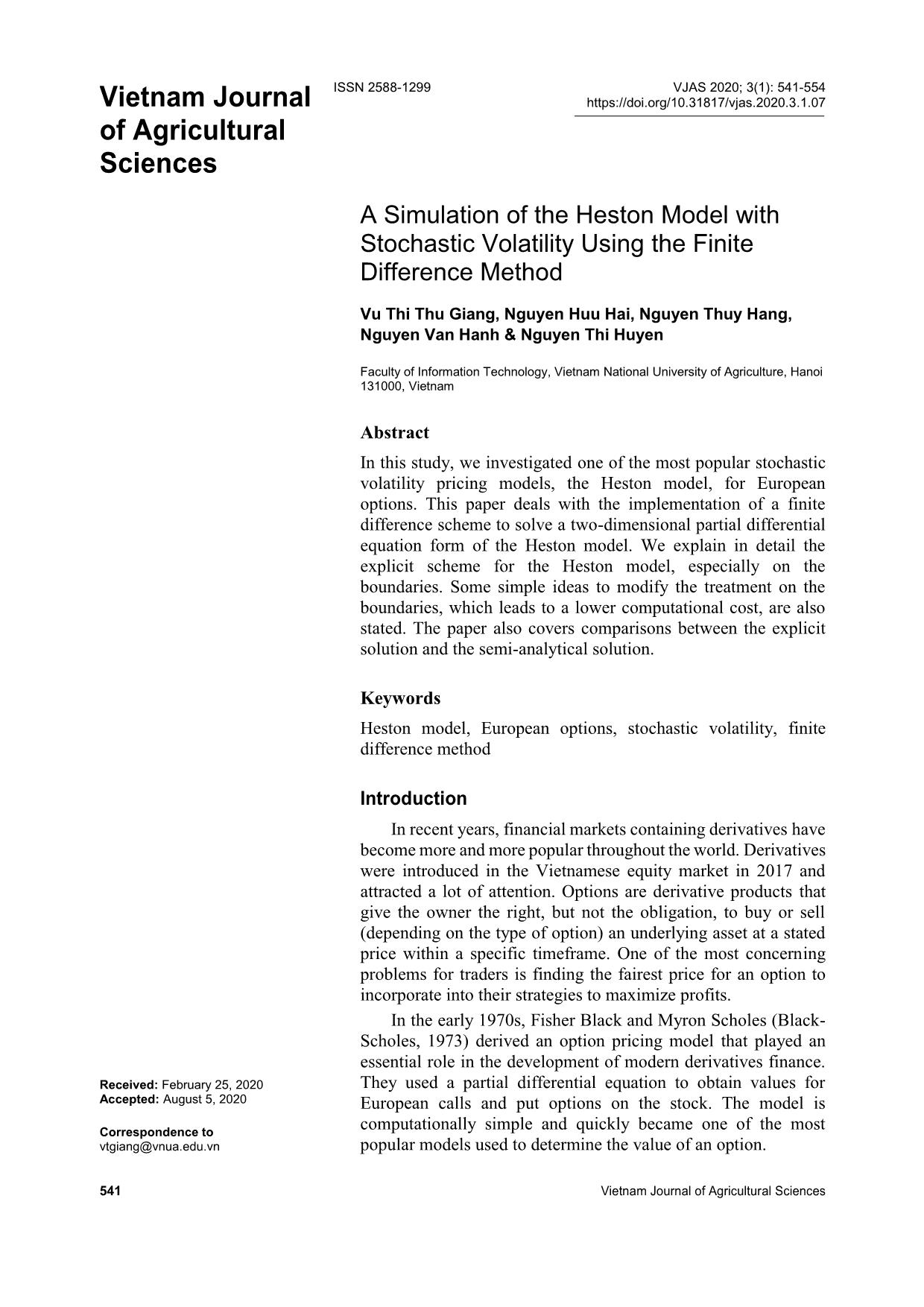
Trang 1
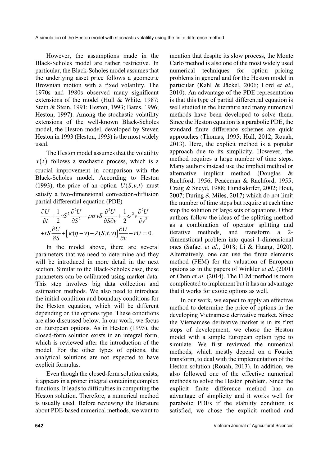
Trang 2
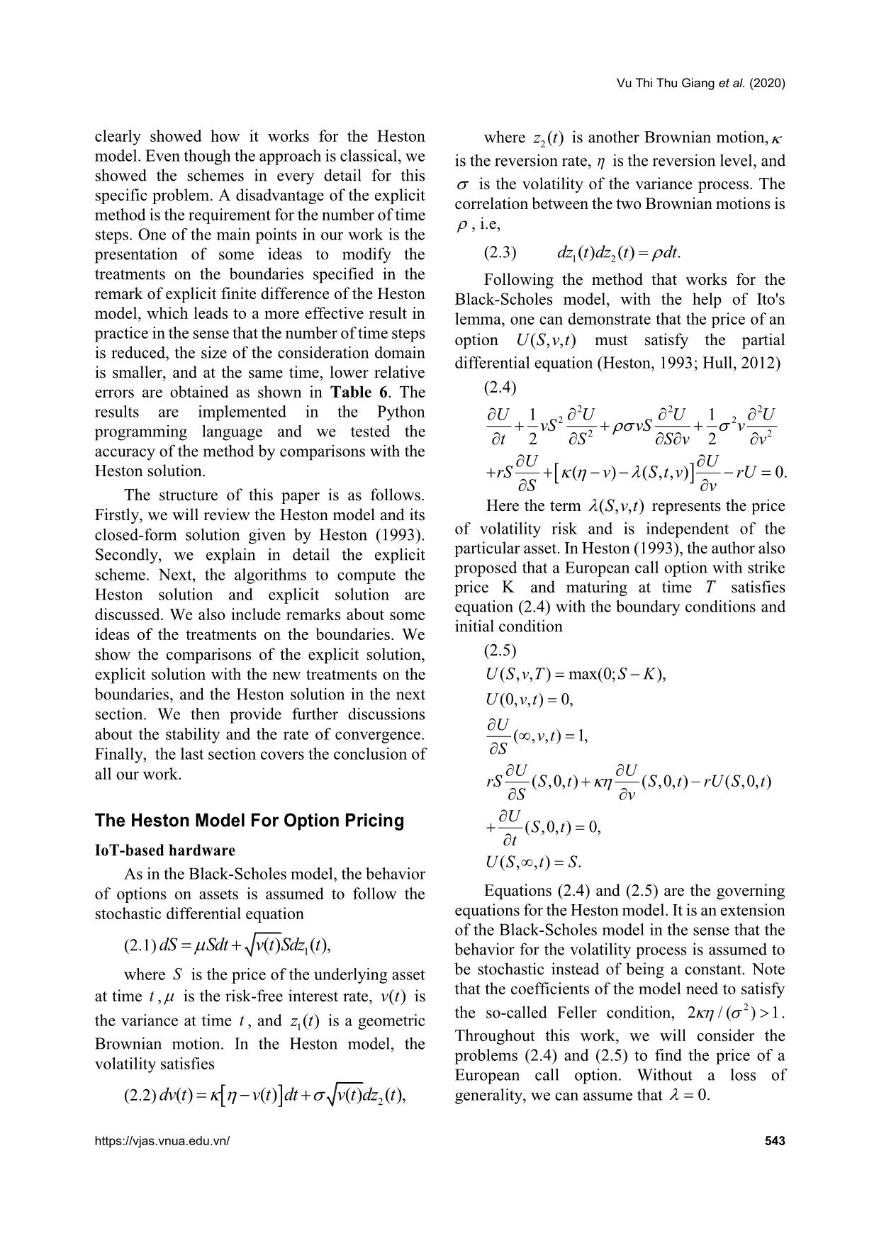
Trang 3
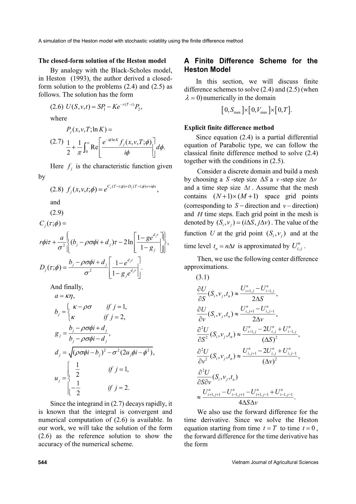
Trang 4
Trang 5
Trang 6
Trang 7
Trang 8
Trang 9
Trang 10
Tải về để xem bản đầy đủ
Bạn đang xem 10 trang mẫu của tài liệu "A simulation of the heston model with stochastic volatility using the finite difference method", để tải tài liệu gốc về máy hãy click vào nút Download ở trên
Tóm tắt nội dung tài liệu: A simulation of the heston model with stochastic volatility using the finite difference method
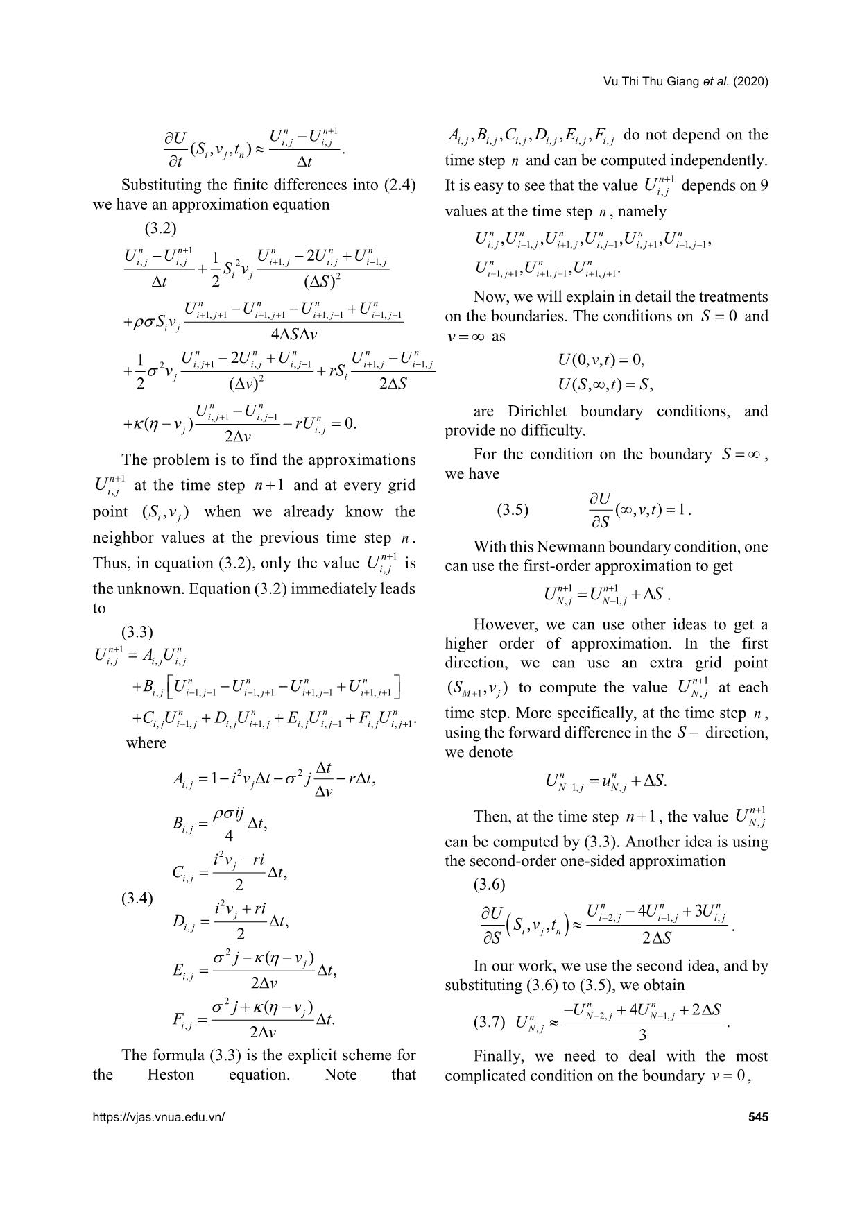
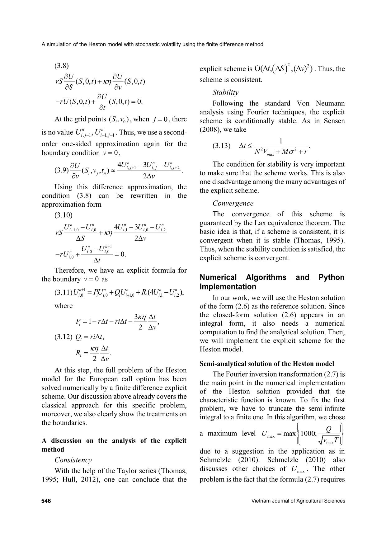
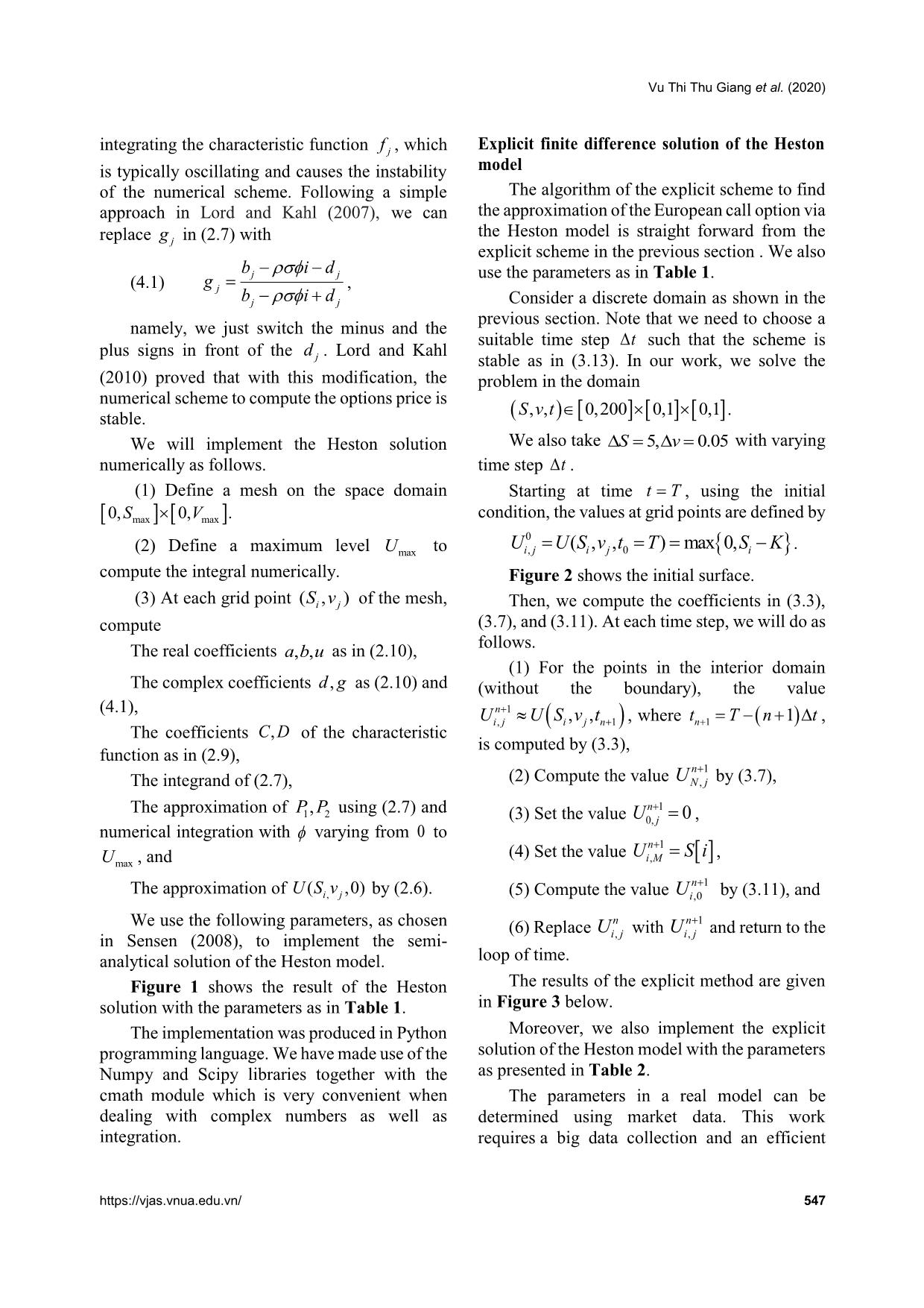
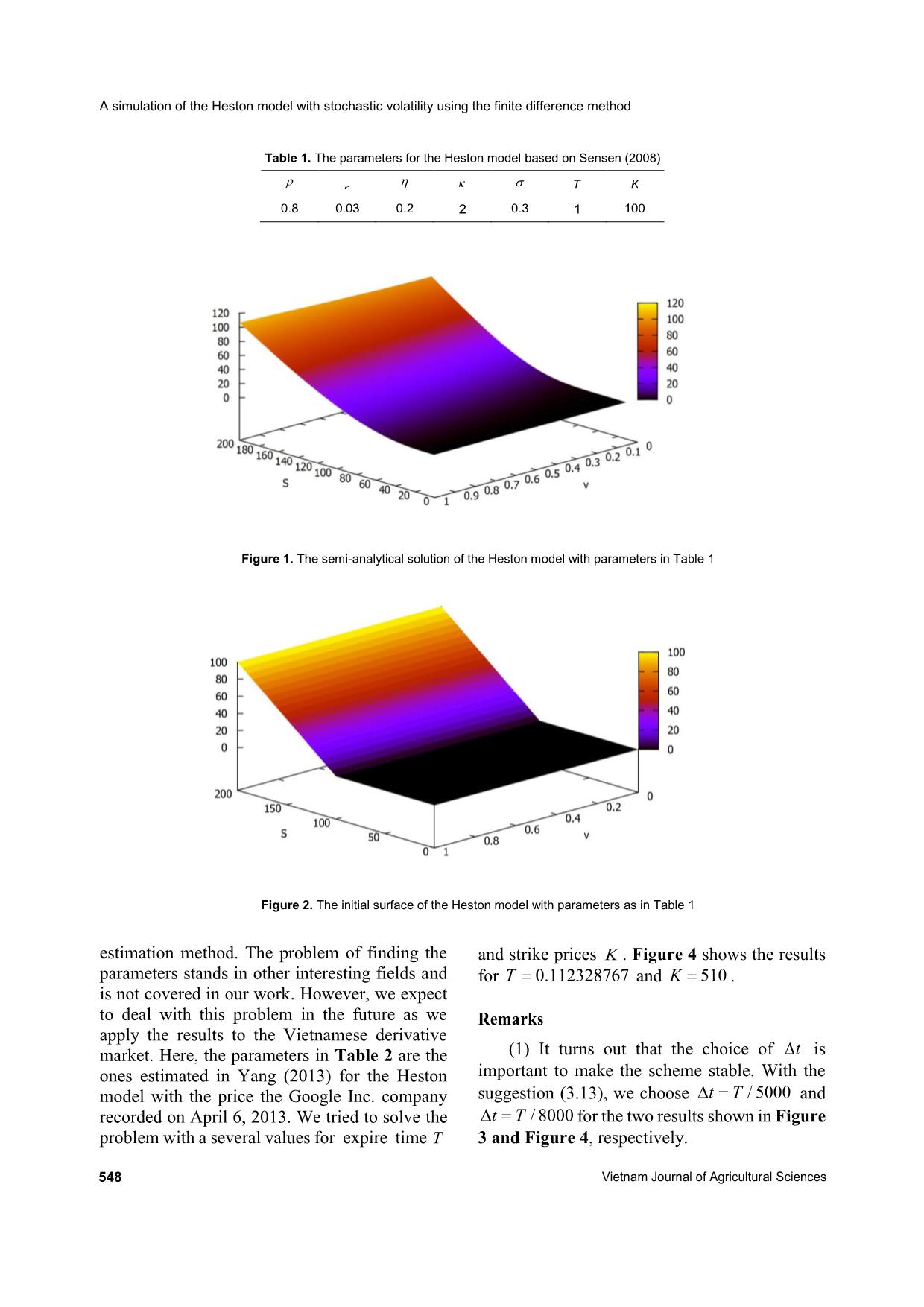
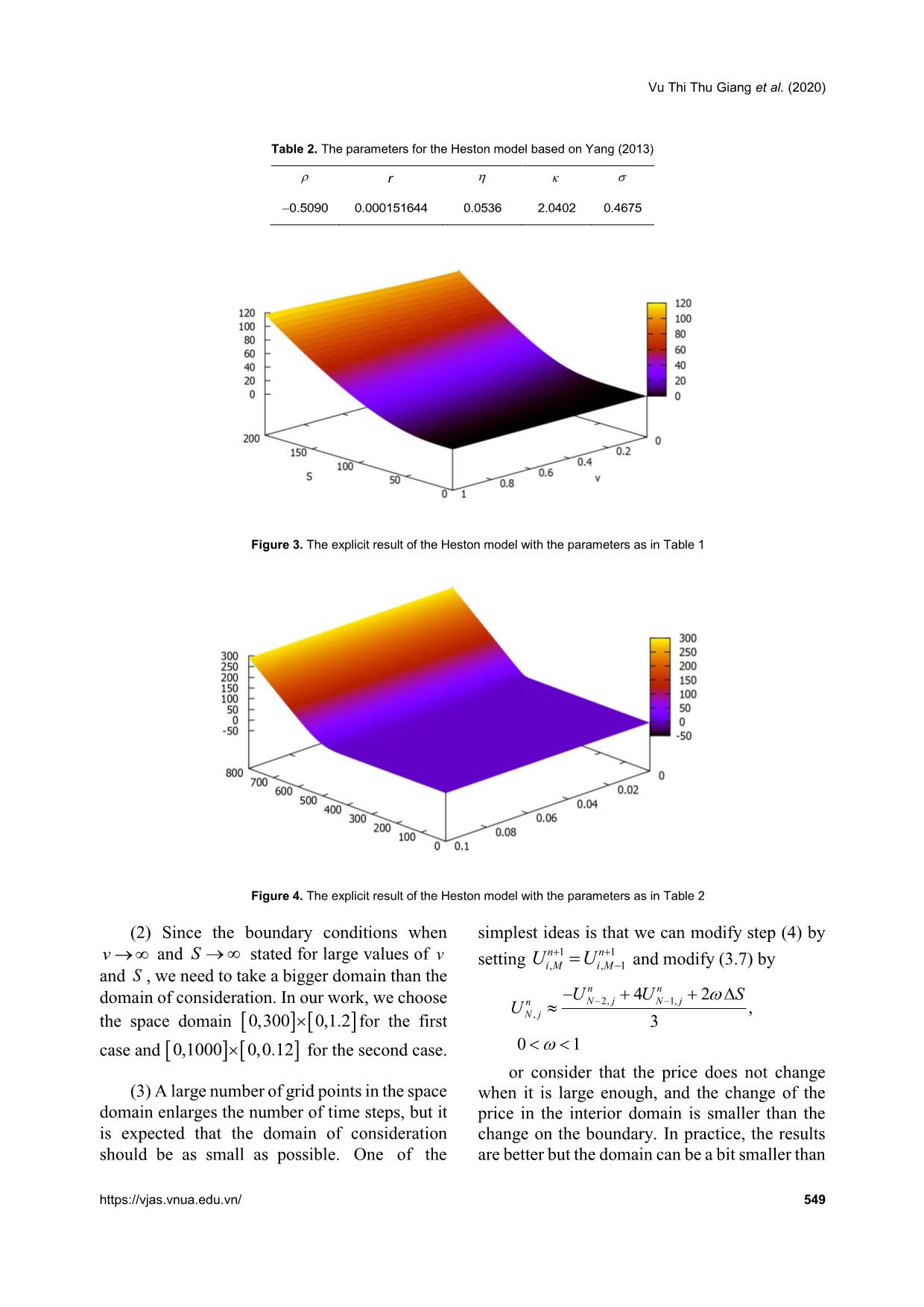
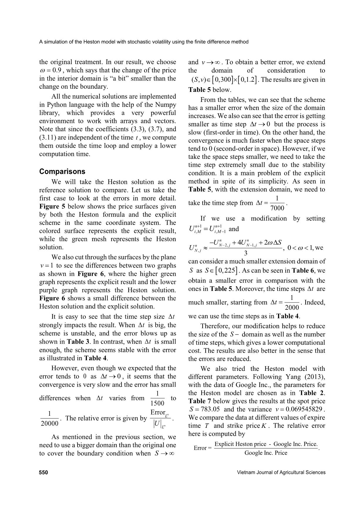
Figure 1 shows the result of the Heston The results of the explicit method are given solution with the parameters as in Table 1. in Figure 3 below. The implementation was produced in Python Moreover, we also implement the explicit programming language. We have made use of the solution of the Heston model with the parameters Numpy and Scipy libraries together with the as presented in Table 2. cmath module which is very convenient when The parameters in a real model can be dealing with complex numbers as well as determined using market data. This work integration. requires a big data collection and an efficient https://vjas.vnua.edu.vn/ 547 A simulation of the Heston model with stochastic volatility using the finite difference method Table 1. The parameters for the Heston model based on Sensen (2008) r T K 0.8 0 . 0 3 0.2 2 0.3 1 100 Figure 1. The semi-analytical solution of the Heston model with parameters in Table 1 Figure 2. The initial surface of the Heston model with parameters as in Table 1 estimation method. The problem of finding the and strike prices K . Figure 4 shows the results parameters stands in other interesting fields and for T 0.112328767 and K 510 . is not covered in our work. However, we expect to deal with this problem in the future as we Remarks apply the results to the Vietnamese derivative (1) It turns out that the choice of t is market. Here, the parameters in Table 2 are the ones estimated in Yang (2013) for the Heston important to make the scheme stable. With the suggestion (3.13), we choose tT/ 5000 and model with the price the Google Inc. company recorded on April 6, 2013. We tried to solve the tT/ 8000 for the two results shown in Figure problem with a several values for expire time T 3 and Figure 4, respectively. 548 Vietnam Journal of Agricultural Sciences Vu Thi Thu Giang et al. (2020) Table 2. The parameters for the Heston model based on Yang (2013) r 0 . 5 0 9 0 0 . 0 0 0 1 5 1 6 4 4 0 . 0 5 3 6 2 . 0 4 0 2 0 . 4 6 7 5 Figure 3. The explicit result of the Heston model with the parameters as in Table 1 Figure 4. The explicit result of the Heston model with the parameters as in Table 2 (2) Since the boundary conditions when simplest ideas is that we can modify step (4) by v and S stated for large values of v nn 11 setting UUi,,1 Mi M and modify (3.7) by and S , we need to take a bigger domain than the nn domain of consideration. In our work, we choose UUSN 2,1, jN42 j U n , the space domain 0,300 0,1.2for the first Nj, 3 case and 0,10000,0.12 for the second case. 01 or consider that the price does not change (3) A large number of grid points in the space when it is large enough, and the change of the domain enlarges the number of time steps, but it price in the interior domain is smaller than the is expected that the domain of consideration change on the boundary. In practice, the results should be as small as possible. One of the are better but the domain can be a bit smaller than https://vjas.vnua.edu.vn/ 549 A simulation of the Heston model with stochastic volatility using the finite difference method the original treatment. In our result, we choose and v . To obtain a better error, we extend 0.9 , which says that the change of the price the domain of consideration to in the interior domain is “a bit” smaller than the (,)0,3000,1.2Sv . The results are given in change on the boundary. Table 5 below. All the numerical solutions are implemented From the tables, we can see that the scheme in Python language with the help of the Numpy has a smaller error when the size of the domain library, which provides a very powerful increases. We also can see that the error is getting environment to work with arrays and vectors. smaller as time step t 0 but the process is Note that since the coefficients (3.3), (3.7), and slow (first-order in time). On the other hand, the (3.11) are independent of the time t , we compute convergence is much faster when the space steps them outside the time loop and employ a lower tend to 0 (second-order in space). However, if we computation time. take the space steps smaller, we need to take the time step extremely small due to the stability Comparisons condition. It is a main problem of the explicit We will take the Heston solution as the method in spite of its simplicity. As seen in reference solution to compare. Let us take the Table 5, with the extension domain, we need to first case to look at the errors in more detail. 1 take the time step from t . Figure 5 below shows the price surfaces given 7000 by both the Heston formula and the explicit If we use a modification by setting scheme in the same coordinate system. The nn 11 colored surface represents the explicit result, UUiMiM,,1 and while the green mesh represents the Heston UUSnn42 solution. U n NjNj 2,1, , 01, we Nj, 3 We also cut through the surfaces by the plane can consider a much smaller extension domain of v 1 to see the differences between two graphs as shown in Figure 6, where the higher green S as S 0,225 . As can be seen in Table 6, we graph represents the explicit result and the lower obtain a smaller error in comparison with the purple graph represents the Heston solution. ones in Table 5. Moreover, the time steps t are Figure 6 shows a small difference between the 1 much smaller, starting from t . Indeed, Heston solution and the explicit solution. 2000 It is easy to see that the time step size t we can use the time steps as in Table 4. strongly impacts the result. When t is big, the Therefore, our modification helps to reduce scheme is unstable, and the error blows up as the size of the S domain as well as the number shown in Table 3. In contrast, when t is small of time steps, which gives a lower computational enough, the scheme seems stable with the error cost. The results are also better in the sense that as illustrated in Table 4. the errors are reduced. However, even though we expected that the We also tried the Heston model with error tends to 0 as t 0 , it seems that the different parameters. Following Yang (2013), convergence is very slow and the error has small with the data of Google Inc., the parameters for 1 the Heston model are chosen as in Table 2. differences when t varies from to 1500 Table 7 below gives the results at the spot price S 783.05 and the variance v 0.069545829 . 1 Error . The relative error is given by L . We compare the data at different values of expire 20000 U L time T and strike price K . The relative error As mentioned in the previous section, we here is computed by Explicit Heston price - Google Inc. Price. need to use a bigger domain than the original one Error = . to cover the boundary condition when S Google Inc. Price 550 Vietnam Journal of Agricultural Sciences Vu Thi Thu Giang et al. (2020) Figure 5. The Heston solution and the explicit solution of the Heston model with parameters as in Table 1. Figure 6. The cut at v 1 of the surfaces in Figure 5. Table 3. The L error when the scheme is unstable t Error (in L norm) 1 8.33.10136 500 1 4.08.10279 1000 1 11.126266 1200 We denote the explicit Heston price by applied efficiently to the Heston model with H price . We can see that the scheme can be different kinds of parameters. https://vjas.vnua.edu.vn/ 551 A simulation of the Heston model with stochastic volatility using the finite difference method Table 4. The L error and the relative error when the scheme is stable, with S 5, v 0.05,( S , v ) 0,200 0,1 t Error (in L norm) Relative Error 1 1 1 . 1 2 5 4 6 3 1 0 . 4 6 5 9 % 1500 1 1 1 . 1 2 3 8 5 6 1 0 . 4 6 4 4 % 3000 1 1 1 . 1 2 3 2 0 8 1 0 . 4 6 3 8 % 4500 1 1 1 . 1 2 3 0 5 3 1 0 . 4 6 3 6 % 6000 1 1 1 . 1 2 2 4 9 1 1 0 . 4 6 3 1 % 20000 Table 5. The L error and the relative error when the scheme is stable, with SvS5,0.05, v (,)0,3000,1.2 t Error (in L norm) Relative Error 1 5 . 9 5 7 4 8 3 1 3 5 . 6 0 4 3 % 7000 1 5 . 9 5 7 5 3 4 1 9 5 . 6 0 4 4 % 10000 1 5.95753075 5.6043% 20000 Table 6. The L error and the relative error when the modification scheme is stable, with SvS5,0.05, v ( , )0,2250,1.2 t Error (in L norm) Relative Error 1 4.325400 4.6090% 2000 1 4.325450 4.6090% 3000 1 4.325489 4.6091% 5000 Table 7. A comparison between the explicit solution of the Heston model with the parameters as in Table 2 and the data of Google Inc. at the spot price S 783.05 and the variance v 0.069545829 Google Inc. Expire time T Strike price K H - price Error (%) price 0.112328767 510 272.90 272.5087508 0.1539 0.112328767 590 193.25 192.5350415 0.3699 0.457534247 395 388.30 387.5296684 0.1983 0.457534247 410 373.40 372.5333392 0.2320 0.783561644 395 389.70 387.5881280 0.5419 0.783561644 410 375.00 372.6184232 0.6350 552 Vietnam Journal of Agricultural Sciences Vu Thi Thu Giang et al. (2020) Conclusions Heston S. (1993). A closed‐form solution for options with stochastic volatility. The Review of Financial Studies. In our work, the explicit finite difference 6: 327-343. scheme with some simple modifications on the Heston S. (1997). A simple new formula for options with boundaries have been applied to the Heston stochastic volatility. Working paper. Olin J. M. School pricing model with European options. Our results of Business. Washington University. show that the explicit scheme with the Hout K. J. in ’t (2007). ADI schemes in the numerical solution of the Heston PDE. Numerical Analysis and modifications is simple, easy to apply, and gives Applied Mathematics. AIP Conference Proceedings. a better approximation to the Heston solution in 936: 10-14. DOI: 10.1063/1.2790085 comparison with the classical method. However, Hull J. C. & White A. (1987). The pricing of options on the scheme still has the disadvantage of stability assets with stochastic volatility. Journal of Finance. conditions. To overcome this disadvantage, some 42: 281‐300. authors developed the alternative direction Hull J. C. (2012). Options, futures and other derivatives (8th ed.). Prentice-Hall. Upper Saddle River. implicit (ADI) scheme, which is a kind of mixed Hundsdorfer W. (2002). Accuracy and stability of splitting explicit-implicit scheme. The ADI scheme is with Stabilizing Corrections. Applied Numerical unconditionally stable. Nevertheless, it is more Mathematics. 42: 213‐233. complicated in comparison with the explicit Kahl C. & Jäckel P. (2006). Fast strong approximation method. Furthermore, the ADI scheme must be Monte Carlo schemes for stochastic volatility models. used with care since a high dimensional matrix Quantitative Finance. 6: 513-536. Lewis A. (2000). Option Valuation under Stochastic appears in a linear system of equations and an Volatility: With Mathematica Code. Finance Press. efficient solver is needed. In future work, we Newport Beach. expect to apply this method in an efficient way to Li H. & Huang Z. (2020) An iterative splitting method for the Heston model with more complicated options pricing European options under the Heston model. types such as the American option and Barrier Applied Mathematics and Computation. DOI: 10.1016/j.amc.2020.125424. option. Besides, the parameter estimation and the Lord R. & Kahl C. (2007). Optimal Fourier Inversion in application of this scheme in the Vietnamese Semi-Analytical Option Pricing. Tinbergen Institute derivative market is also a problem of interest. Discussion Paper 2006-066(2). Retrieved from https://ssrn.com/abstract=921336 or on September References 20, 2019. Lord R., Koekkoek R. & van Dijk D. (2010). A comparison Bates D. S. (1996). Jumps and stochastic volatility: of biased simulation schemes for stochastic volatility Exchange rate processes implicit in Deutsche Mark models. Quantitative Finance. 10: 177-194. options. Review of Financial Studies. 9(1): 69-107. Merton R. (1973). The theory of rational option pricing. Black F. & Scholes M. (1973). The Pricing of Options and Bell Journal of Economics and Management Science. Corporate Liabilities. Journal of Political Economy. 4: 141-183. 81(3): 637-654. Merton R. (1976). Option pricing when underlying stock Chen X., Burkardt J. & Gunzburger M. (2014). High returns are discontinuous. Journal of Financial accuracy finite element methods for option pricing Economics. 3: 125-144. under Heston’s stochastic volatility model. Florida Peaceman D. W. & Rachford H. H. (1955). The numerical State University. solution of parabolic and elliptic differential equations. Craig I. J. D. & Sneyd A. D. (1988). An alternating‐ Journal of the Society for Industrial and Applied direction implicit scheme for parabolic equations with Mathematics. 3: 28‐41. mixed derivatives. Computer & Mathematics with Rouah F. D. (2013). The Heston Model and Its Extensions Applications. 16(4): 341-350. in Matlab and C#. John Wiley & Sons, Ltd. Douglas J. & Rachford H. H. (1956). On the numerical Safaei M., Neisy A. & Nematollahi N. (2018). New solution of heat conduction problems in two and three splitting scheme for pricing American options under space variables. Transactions of the American the Heston model. Computational Economics. 52(2): Mathematical Society. 82: 421‐439. 405-420. During B. & Miles J. (2017). High-order ADI scheme for Schmelzle M. (2010). Option pricing formulae using option pricing in stochastic volatility models. Journal of Fourier transform: Theory and application. Working Computational and Applied Mathematics. 316:109-121. paper. Retrieved from https://vjas.vnua.edu.vn/ 553 A simulation of the Heston model with stochastic volatility using the finite difference method https://pfadintegral.com/docs/Schmelzle2010%20Fou Thomas J. W. (1995). Numerical Partial Differential rier%20Pricing.pdf on September 25, 2019. Equations: Finite Difference Methods. New York, Sensen L. (2008). Finite Difference Schemes for Heston Springer-Verlag. Model. Thesis. Retrieved from Winkler G., Apel T. & Wystup U. (2001). Valuation of options https://core.ac.uk/download/pdf/97116.pdf on in Heston’s stochastic volatility model using finite January 10, 2019. element methods. Foreign Exchange Risk. 283-303. Stein E. M. & Stein J. C. (1991). Stock price distributions Yang Y. (2013). Valuing a European option with the with stochastic volatility: an analytic approach. Heston model. Master’s Thesis. Rochester Institute of Review of Financial Studies. 4(4): 727-752. Technology. 554 Vietnam Journal of Agricultural Sciences
File đính kèm:
 a_simulation_of_the_heston_model_with_stochastic_volatility.pdf

