Nonstandard finite difference schemes for solving a modified epidemiological model for computer viruses

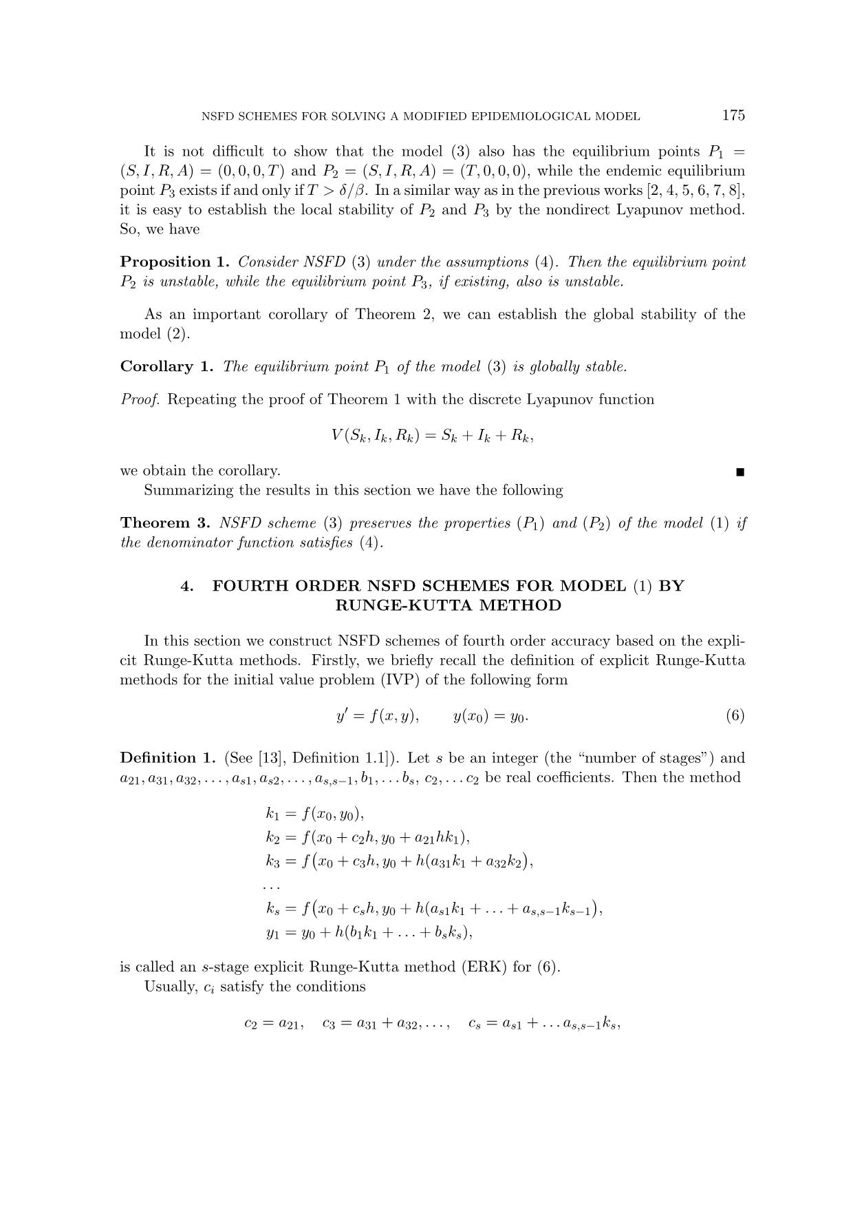
we have the eigenvalue
µ∗ of J∗. Obviously, µ∗ > 1 because λ∗ > 0. Hence, the point P3 is unstable.
Now we consider the stability of the equilibrium point P1. Recall that σ(J(P1)) =
{−αSAT,−αIAT − δ,−σ, 0}. Corresponding to the eigenvalue λ = 0 of J we have the
eigenvalue µ = 1 of J∗. Nevertheless, as in the continuous case, this eigenvalue does not
imply bifurcation or central manifold for the model [25], representing only the fact that one
equation can be expressed as a linear combination of the other three. Corresponding to the
eigenvalues λ1 = −αSAT, λ2 = −αIAT − δ, λ3 = −σ of J we have the following eigenvalues
of J∗
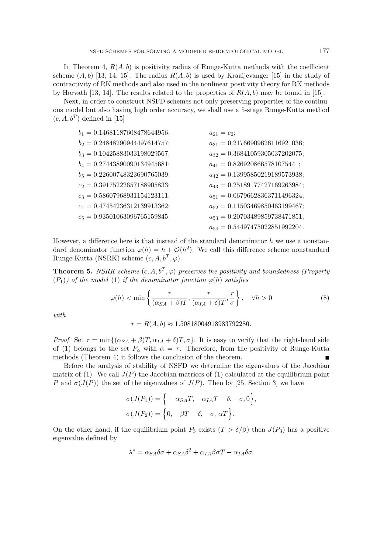
P(z) = a5z5 + 1
24
z4 +
1
6
z3 +
1
2
z2 + z + 1, z = ϕλ1,
P(z) = a5z5 + 1
24
z4 +
1
6
z3 +
1
2
z2 + z + 1, z = ϕλ2,
P(z) = a5z5 + 1
24
z4 +
1
6
z3 +
1
2
z2 + z + 1, z = ϕλ3.
By Lyapunov theorem [10, 16], the necessary and sufficient condition for P1 to be locally
stable is |P(λi)| < 1, i = 1, 2, 3. This is equivalent to the system
a5ϕ
5(λi)
5 +
1
24
ϕ4(λi)
4 +
1
6
ϕ3(λi)
3 +
1
2
ϕ2(λi)
2 + ϕλi < 0, (9)
Pi(ϕ) := a5ϕ5(λi)5 + 1
24
ϕ4(λi)
4 +
1
6
ϕ3(λi)
3 +
1
2
ϕ2(λi)
2 + ϕλi > −2, (10)
for i = 1, 2, 3. We also see that (9) is equivalent to
Qi := a5ϕ4(λi)5 + 1
24
ϕ3(λi)
4 +
1
6
ϕ2(λi)
3 +
1
2
ϕ(λi)
2 + λi < 0.
NSFD SCHEMES FOR SOLVING A MODIFIED EPIDEMIOLOGICAL MODEL 179
It is easy to see that Pi(ϕ) → 0 as ϕ → 0 and Qi(ϕ) → λi < 0 as ϕ → 0. Therefore, from
the definition of limit of a function it follows that there exists a number τ∗ > 0 such that
Pi(ϕ) > −2 and Qi(ϕ) < 0 for any ϕ < τ∗, or in other words, (9) and (10) are satisfied if
ϕ < τ∗. Thus, the theorem is proved. 
Remark 1. In Theorem 6, the number τ∗ can be determined as τ∗ = mini=1,2,3{pi, qi},
where pi and qi are minimal root of the polynomials Pi(ϕ) and Qi(ϕ), respectively.
Summarizing the results in this section we obtain
Theorem 7. NSRK (5) preserves the properties (P1) and (P2) of (1) if the denominator
function satisfies the condition
ϕ(h) < min
{
r
(αSA + β)T
,
r
(αIA + δ)T
,
r
σ
, τ∗
}
, ∀h > 0. (11)
Clearly, the denominator function ϕ(h) = h does not satisfy (11). Therefore, we should
select the denominator function satisfying (11) and not influencing on the accuracy order of
the original Runge-Kutta methods. For doing this we need the following
Corollary 2. NSRK (c, A, bT , ϕ) is of fourth order of accuracy if the denominator function
satisfies the condition
ϕ(h) = h+O(h5). (12)
Thus, we have to select denominator functions satisfying simultaneously (11) and (12).
The selection of such functions is an interesting and important problem. Analogously as in
the recent work [6], we select denominator functions of the form
ϕ(h) = (1− θ(h))1− e
−τh
τ
+ θ(h)he−µh
m
, θ(h) = 1 +O(hp).
5. NUMERICAL SIMULATIONS
In this section we report the results of some numerical simulations in order to confirm the
validity of obtained theoretical results and to demonstrate the efficiency of designed NSFD
schemes. It should be emphasized that all numerical simulations in [2, 4, 5, 6, 7, 8, 19, 20,
21, 22] showed that standard difference schemes do not preserve essential properties of the
corresponding continuous models.
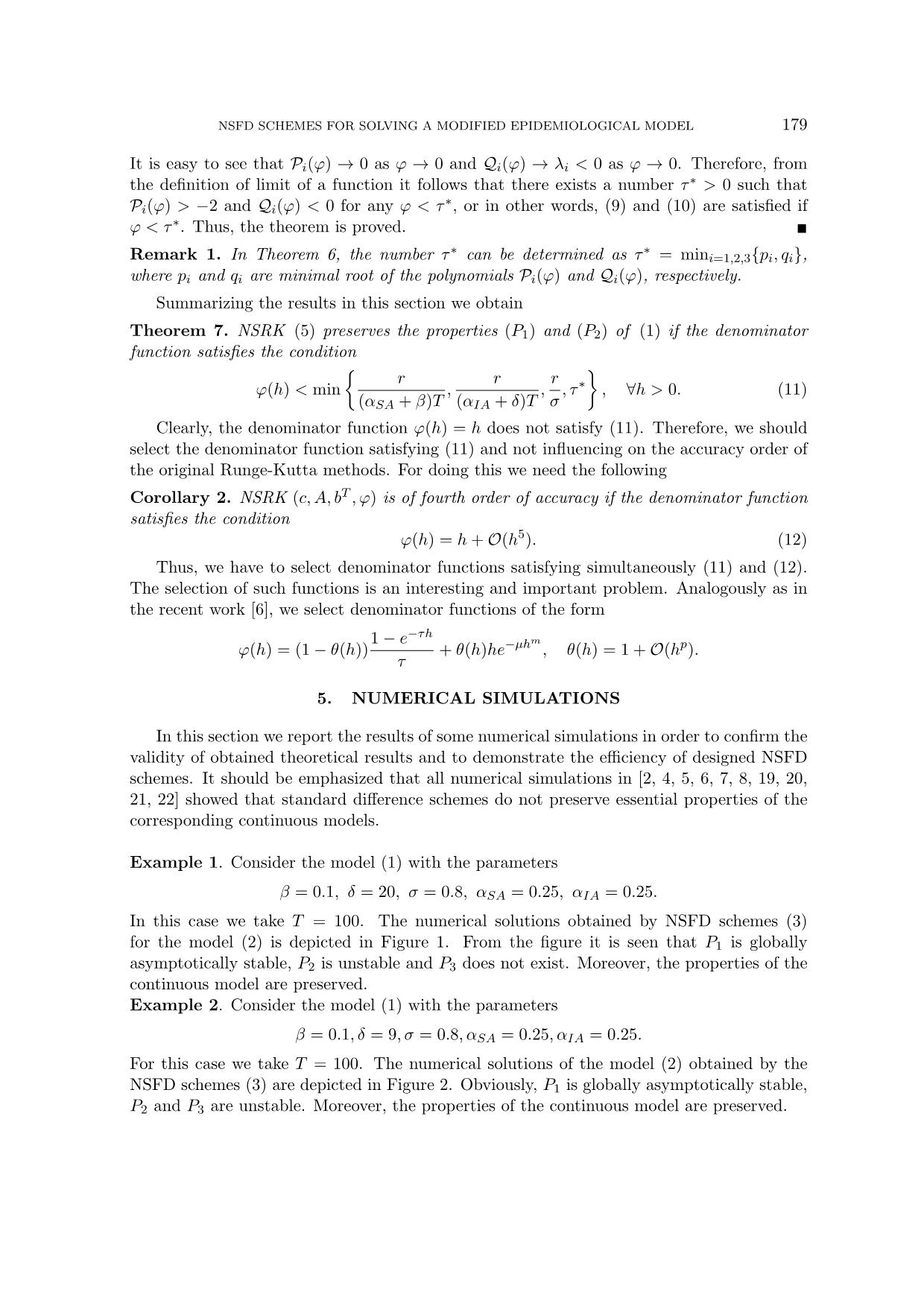
Example 1. Consider the model (1) with the parameters
β = 0.1, δ = 20, σ = 0.8, αSA = 0.25, αIA = 0.25.
In this case we take T = 100. The numerical solutions obtained by NSFD schemes (3)
for the model (2) is depicted in Figure 1. From the figure it is seen that P1 is globally
asymptotically stable, P2 is unstable and P3 does not exist. Moreover, the properties of the
continuous model are preserved.
Example 2. Consider the model (1) with the parameters
β = 0.1, δ = 9, σ = 0.8, αSA = 0.25, αIA = 0.25.
For this case we take T = 100. The numerical solutions of the model (2) obtained by the
NSFD schemes (3) are depicted in Figure 2. Obviously, P1 is globally asymptotically stable,
P2 and P3 are unstable. Moreover, the properties of the continuous model are preserved.
180 DANG QUANG A, HOANG MANH TUAN, DANG QUANG LONG
P1
P2
100
800
5
60
10
60
15
50
S
20R
40
25
40
30
I
30
35
40
20 20
10 00
Figure 1. Numerical solutions obtained by NSFD schemes (3) with ϕ(h) = 1−e−h and h = 1
Example 3. Accuracy and computation time of schemes
Consider the model (1) with the parameters
β = 0.01, δ = 0.02, σ = 0.5, αSA = 0.025, αIA = 0.02
and the initial values (20, 30, 20, 30). We report the errors of the NSFD and NSRK (c, A, bT , ϕ).
For comparison we also consider the method proposed by Wood and Koruharov in [27], which
preserves the positivity and stability of dynamical systems based on nonlocal discretization.
The denominator functions used for NSFD scheme (3), NSRK scheme and Wood and Kor-
uharov’s scheme, respectively are
ϕ(h) =
1− e−0.6h
0.6
, ϕ(h) = e−h
8
he−0.0001h
6
+
(1− e−h8)(1− e−1.1h)
1.1
, ϕ(h) =
1− e−0.6h
0.6h
.
Since it is impossible to find the exact solution of the model, as a benchmark we use the
numerical solution obtained by 11-stage Runge-Kutta method [9]. The benchmark solution
is depicted in Figure 3. From the figure it is seen that the components of the solution change
very quickly in a short time from the starting points, after that they become stable. The
differential problem in this case is stiff. Table 1 provides the errors and the rates of the NSFD
NSFD SCHEMES FOR SOLVING A MODIFIED EPIDEMIOLOGICAL MODEL 181
P2
P1
P3
1000
8050
10
20
6040
S
30R
30
40
I
40
50
20
60
2010
00
Figure 2. Numerical solutions obtained by NSFD schemes (3) with ϕ(h) = e−h8he−0.0001h6 +
(1− e−h8)(1− e−1.1h)/1.1 and h = 1
scheme, Wood and Koruharov’s (W-K’s) scheme and NSRK scheme for different stepsizes.
There errors are computed by the formula
err = max
k
{|Sk − S(tk)|+ |Ik − I(tk)|+ |Rk −R(tk)|+ |Ak −A(tk)|},
where Uk and U(tk) are the solutions obtained by a scheme and the benchmark solution,
respectively. Besides, rate := log h1
h2
(err1/err2) (see [1, Example 4.1]) is an approximation for
accuracy order of the schemes. In the last column of Table 1 (rate of NSRK scheme), we see
an unexpected phenomenon, when h is small the rates decrease. A similar phenomenon also
was indicated in [1, Example 4.1]) when studying explicit standard Runge-Kutta methods.
The reason of this is that the rounding errors generally increase as h decreases.
The computation time is given in Table 2. From the tables we see that NSFD (3)
has better accuracy and faster then the Wood and Koruharov’s scheme. The reason is
that at each step Wood and Koruharov’s scheme needs to consider the sign of the right-
hand sides for choosing appropriate discretization. NSRK scheme has the best accuracy but
the computation time is largest because at each step it requires computation of values of
stages Ki. However, to obtain the solution of high order of accuracy the use of NSRK is
more efficient than the use of extrapolation, which combines the solutions of first order of
182 DANG QUANG A, HOANG MANH TUAN, DANG QUANG LONG
0 10 20 30 40 50
t
0
5
10
15
20
S
0 10 20 30 40 50
t
0
5
10
15
I
0 10 20 30 40 50
t
0
2
4
6
8
10
R
0 10 20 30 40 50
t
0
10
20
30
40
A
Figure 3. Benchmark solution obtained by RK8 with h = 10−5
Table 1. Errors and rates of the schemes
Stepsize NSFD scheme Rate W-K’s scheme Rate NSRK scheme Rate
0.25 6.463466701595602 7.713254298410573 1.2780e-04
0.2 5.243459924068896 0.9374 6.056566836376636 1.0836 2.7012e-05 6.9650
0.15 3.989310828795733 0.9502 4.459865753797996 1.0638 5.5149e-06 5.5229
0.1 2.698912044130053 0.9638 2.920085782158711 1.0445 9.2956e-07 4.3913
0.05 1.369838435912756 0.9784 1.434358023863455 1.0256 5.6487e-08 4.0405
0.001 0.027798934145437 0.9963 0.028200224634866 1.0044 1.7708e-12 2.6509
0.00001 0.000278071734776 0.9999 0.000281905383956 1.0001 9.3258e-15 1.1392
accuracy. The advantage of NSRK is that it has high order of accuracy for small stepsizes
and preserves the properties of the model for large stepsizes. Moreover, it is explicit, easy
to be programmed.
6. CONCLUSIONS
In this paper we have constructed two families of NSFD schemes preserving the essential
properties of a computer virus spread model. They are positivity, boundedness and local
stability. Besides, the first NSFD schemes are globally stable, the second NSFD schemes are
NSFD SCHEMES FOR SOLVING A MODIFIED EPIDEMIOLOGICAL MODEL 183
Table 2. Computation times of the schemes in seconds
Stepsize NSFD scheme (3) W-Ks scheme NSRK scheme
0.2 0.001897 0.027662 0.048200
0.1 0.001942 0.012523 0.043975
0.05 0.002224 0.016025 0.064037
0.01 0.006202 0.066508 0.306687
0.005 0.006793 0.118272 0.632497
0.001 0.028386 0.616064 2.859388
0.0001 0.210997 5.866315 27.817605
0.00001 2.069937 57.343785 273.413824
of fourth order of accuracy. The numerical simulations confirm the validity of obtained the-
oretical results. Among these constructed schemes, NSFD schemes have advantage in order
of accuracy for small stepsizes and preserves the properties of the corresponding continuous
model for large stepsizes. The method for designing high order, dynamically consistent sche-
mes are applicable to some other applied models. This is the subject of our research in the
future.
ACKNOWLEDGMENT
This work is supported by Vietnam National Foundation for Science and Technology
Development (NAFOSTED) under the grant number 102.01-2017.306.
REFERENCES
[1] Uri M. Ascher, Linda R. Petzold, “Computer methods for ordinary differential equations and
differential algebraic equations”, Society for Industrial and Applied Mathematics, 1998.
[2] Q. A. Dang, M. T. Hoang, “Dynamically consistent discrete metapopulation model”, Journal of
Difference Equations and Applications, vol. 22, pp.1325–1349, 2016.
[3] Q. A. Dang, M. T. Hoang, “Exact finite difference schemes for three-dimensional linear systems
with constant coefficients, Vietnam Journal of Mathematics, vol. 46, no 3, pp. 471-492, 2018.
[4] Q. A. Dang, M. T. Hoang, “Lyapunov direct method for investigating stability of nonstandard
finite difference schemes for metapopulation models”, Journal of Difference Equations and Ap-
plications, vol. 24, pp.15-47, 2018.
[5] Q. A. Dang, M. T. Hoang, “Nonstandard finite difference schemes for a general predator-prey
system”, arXiv:1701.05663 [math.NA] (2018).
[6] Q. A. Dang, M. T. Hoang, “Positive and elementary stable explicit nonstandard Runge-Kutta
methods for a class of autonomous dynamical systems”, arXiv:1710.01421v1 [math.NA] (2017).
[7] Q. A. Dang, M. T. Hoang, “Nonstandard finite difference schemes for numerical simulation
of a metapopulation model using the Lyapunov stability theorem”, The 9th National Confe-
rence on Fundamental and Applied Information Technology Research (FAIR’9), 2017. DOI:
10.1562/vap.2016.00034.
184 DANG QUANG A, HOANG MANH TUAN, DANG QUANG LONG
[8] Q. A. Dang, M. T. Hoang, “Nonstandard finite difference schemes for numerical simulation of
a computer virus propagation model”, The 10th National Conference on Fundamental and
Applied Information Technology Research (FAIR’10), 2018. DOI: 10.15625/vap.2017.00045.
[9] G. J. Cooper, J. H. Verner, “Some explicit Runge-Kutta methods of high order”, SIAM Journal
on Numerical Analysis, vol. 9, pp. 389-405, 1972.
[10] S. Elaydi, An Introduction to Difference Equations, Springer Science+Business Media Inc,
2005.
[11] G. Gonzalez-Parra, A. J. Arenas, B. M. Chen-Charpentier, “Combination of nonstandard sche-
mes and Richardsons extrapolation to improve the numerical solution of population models”, Mat-
hematical and Computer Modelling, vol. 52, pp.1030-1036, 2010.
[12] A. Gerisch, R. Weiner, “The positivity of low-order explicit runge-kutta schemes applied in
splitting methods”, Computers and Mathematics with Applications, vol. 45, pp. 53-67, 2003.
[13] Z. Horvath, “On the positivity step size threshold of Runge-Kutta methods”, Applied Numerical
Mathematics, vol. 53, pp.341-356, 2005.
[14] Z. Horvath, “Positivity of Runge-Kutta methods and diagonally split Runge-Kutta methods”,
Applied Numerical Mathematic, vol. 28, pp.306-326, 1998.
[15] J. F. B. M. Kraaijevanger, “Contractivity of Runge-Kutta methods”, BIT, vol. 31, pp. 482-528,
1991.
[16] H. K. Khalil, Nonlinear Systems (3rd Edition), Prentice Hall, Upper Saddle River, 2002.
[17] J. Martin-Vaquero, A. Martin del Rey, A. H. Encinas, J. D. Hernandez Guillen, A. Queiruga-Dios,
G. Rodriguez Sanchez, “Higher-order nonstandard finite difference schemes for a MSEIR model for
a malware propagation”, Journal of Computational and Applied Mathematics, vol.317, pp.146-
156, 2017.
[18] J. Martin-Vaquero, A. Queiruga-Dios, A. Martin del Rey, A. H. Encinas, J. D. Hernandez
Guillen, G. Rodriguez Sanchez, “Variable step length algorithms with high-order extrapolated non-
standard finite difference schemes for a SEIR model”, Journal of Computational and Applied
Mathematics, vol. 330, pp. 848-854, 2018.
[19] R. E. Mickens, Applications of Nonstandard Finite Difference Schemes, World Scientific,
Singapore, 2000.
[20] R. E. Mickens, Advances in the Applications of Nonstandard Finite Difference Schemes,
World Scientific, Singapore, New Jersey, 2005.
[21] R. E. Mickens, Nonstandard Finite Difference Models of Differential Equations, World Scien-
tific, Singapore, 1994.
[22] R. E. Mickens, “Nonstandard finite difference schemes for differential equations”, Journal of
Difference Equations and Applications, vol. 8, no. 9, pp.823-847, 2005.
[23] W. H. Murray, “The application of epidemiology to computer viruses”, Computers & Security,
vol. 7, no. 2, pp.139-145, 1988.
[24] K. C. Partiadar, “Nonstandard finite difference methods: recent trends and further develop-
ments”, Journal of Difference Equations and Applications, vol. 22, pp.817-849, 2016.
NSFD SCHEMES FOR SOLVING A MODIFIED EPIDEMIOLOGICAL MODEL 185
[25] J. C. Piqueira, V. O. Araujo, “A modified epidemiological model for computer viruses”, Applied
Mathematics and Computation, vol. 213, pp.355-360, 2009.
[26] P. Szor, The art of computer virus research and defense. 1st ed. Addison-Wesley Education
Publishers Inc, 2005.
[27] D. Wood, H. V. Kojouharov, “A class of nonstandard numerical methods for autonomous dyn-
amical systems”, Applied Mathematics Letters, vol. 50, pp.78-82, 2015.
[28] X. Yang, B. K. Mishra, Y. Liu, “Computer virus: theory, model, and methods”, Discrete
Dynamics in Nature and Society, (Article ID 473508) (2012).
[29] L-X. Yang, X. Yang, “A new epidemic model of computer viruses”, Communications in Non-
linear Science and Numerical Simulation, vol. 19, pp. 1935-1944, 2014.
[30] L-X.Yang, X. Yang, “Towards the epidemiological modeling of computer viruses”, Discrete
Dynamics in Nature and Society, (Article ID 259671) (2012).
Received on September 27, 2018
Revised on October 01, 2018