Global dynamics of a computer virus propagation model with feedback controls
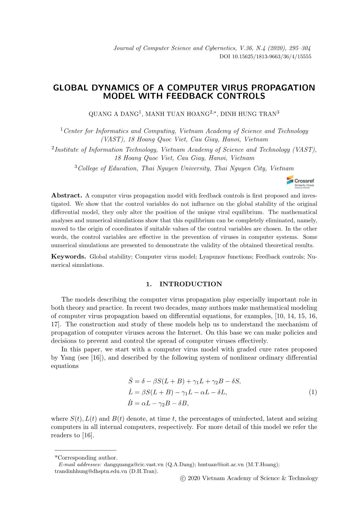
A computer virus propagation model with feedback controls is first proposed and investigated. We show that the control variables do not influence on the global stability of the original
differential model, they only alter the position of the unique viral equilibrium. The mathematical
analyses and numerical simulations show that this equilibrium can be completely eliminated, namely,
moved to the origin of coordinates if suitable values of the control variables are chosen. In the other
words, the control variables are effective in the prevention of viruses in computer systems. Some
numerical simulations are presented to demonstrate the validity of the obtained theoretical results.
Trang 1
Trang 2
Trang 3
Trang 4
Trang 5
Trang 6
Trang 7
Trang 8
Trang 9
Trang 10
Tóm tắt nội dung tài liệu: Global dynamics of a computer virus propagation model with feedback controls
ategies
for protection of computer systems.
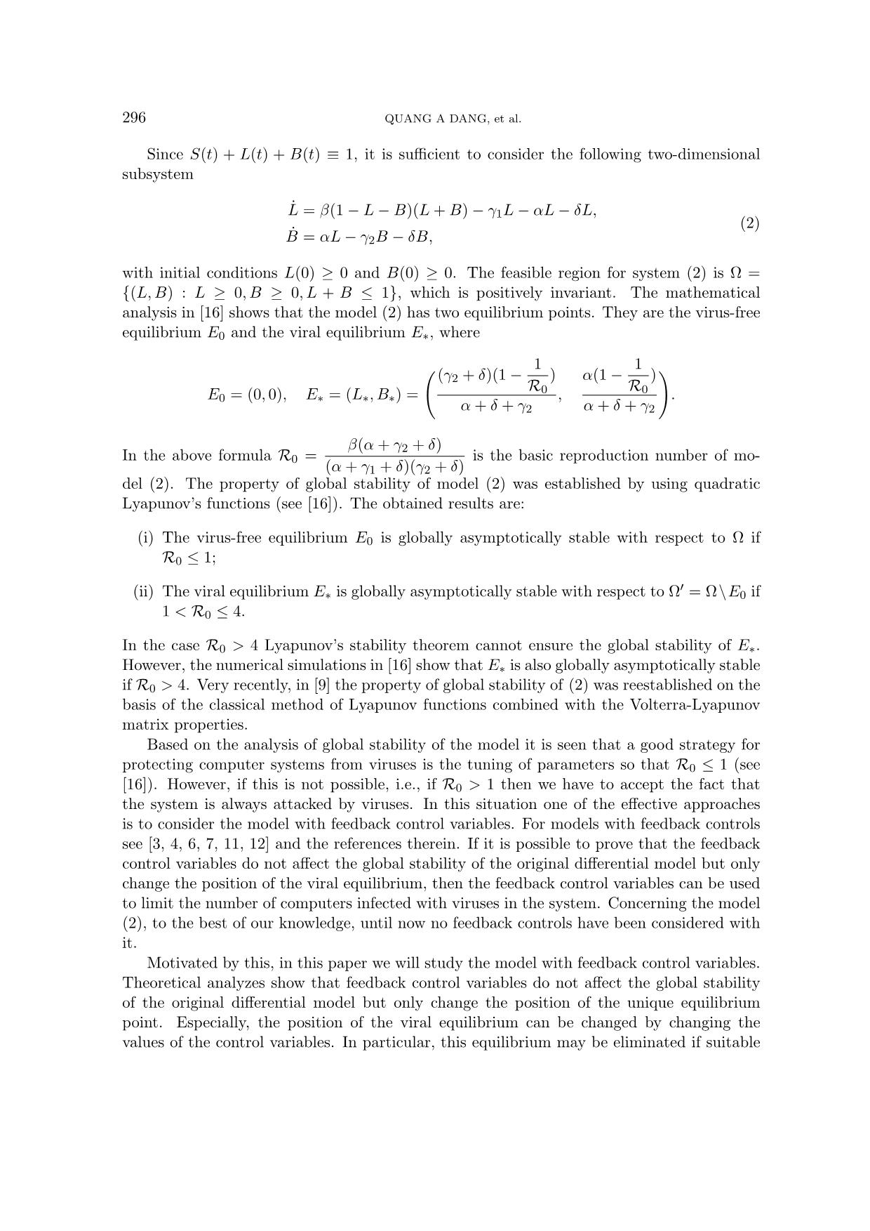
 To analyze the global stability of the proposed model, we use an appropriate Lyapunov for
investigating the global stability of the virus-free equilibrium. Meanwhile, in the context that
the proposed model consists of many equations and contains many parameters, the analysis
of stability of the positive equilibrium point is very difficult because the expressions of this
equilibrium point as well as the associated Jacobian matrix are very complicated. Therefore,
we investigate the global stability of the equilibrium point via numerical simulations. The
numerical simulations agree that if the equilibrium point exists then it is indeed global
stable. This fact completely agrees with the related results of ordinary differential models in
ecology and epidemiology, namely, for the majority of models in these fields, if the positive
equilibrium points exist then they are globally asymptotically stable, i.e,. the models achieve
the robust development (see [1, 2]).
 The paper is organized as follows. In Section 2, a model with feedback controls is pro-
posed. The global stability of the model is investigated in Section 3. Numerical simulations
are presented in Section 4. Finally, some conclusions are given in Section 5.
 2. THE MODEL WITH FEEDBACK CONTROLS
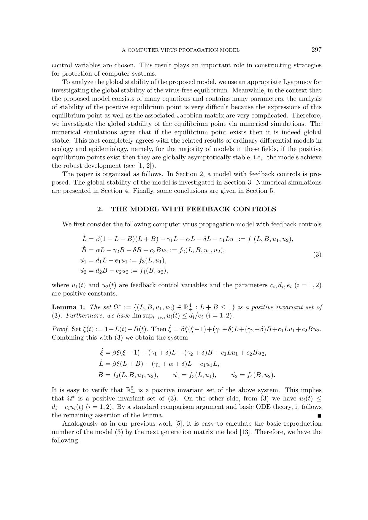
 We first consider the following computer virus propagation model with feedback controls
 L˙ = β(1 − L − B)(L + B) − γ1L − αL − δL − c1Lu1 := f1(L, B, u1, u2),
 B˙ = αL − γ B − δB − c Bu := f (L, B, u , u ),
 2 2 2 2 1 2 (3)
 u˙1 = d1L − e1u1 := f3(L, u1),
 u˙2 = d2B − e2u2 := f4(B, u2),
where u1(t) and u2(t) are feedback control variables and the parameters ci, di, ei (i = 1, 2)
are positive constants.
 ∗ 4
Lemma 1. The set Ω := {(L, B, u1, u2) ∈ R+ : L + B ≤ 1} is a positive invariant set of
(3). Furthermore, we have lim supt→∞ ui(t) ≤ di/ei (i = 1, 2).
Proof. Set ξ(t) := 1−L(t)−B(t). Then ξ˙ = βξ(ξ −1)+(γ1 +δ)L+(γ2 +δ)B +c1Lu1 +c2Bu2.
Combining this with (3) we obtain the system
 ξ˙ = βξ(ξ − 1) + (γ1 + δ)L + (γ2 + δ)B + c1Lu1 + c2Bu2,
 L˙ = βξ(L + B) − (γ1 + α + δ)L − c1u1L,
 B˙ = f2(L, B, u1, u2), u˙1 = f3(L, u1), u˙2 = f4(B, u2).
 5
It is easy to verify that R+ is a positive invariant set of the above system. This implies
 ∗
that Ω is a positive invariant set of (3). On the other side, from (3) we have ui(t) ≤
di − eiui(t)(i = 1, 2). By a standard comparison argument and basic ODE theory, it follows
the remaining assertion of the lemma.
 Analogously as in our previous work [5], it is easy to calculate the basic reproduction
number of the model (3) by the next generation matrix method [13]. Therefore, we have the
following.
298 QUANG A DANG, et al.
Lemma 2. The number
 ∗ β(α + γ2 + δ)
 R0 =
 (α + γ1 + δ)(γ2 + δ)
is the basic reproduction number of model (3).
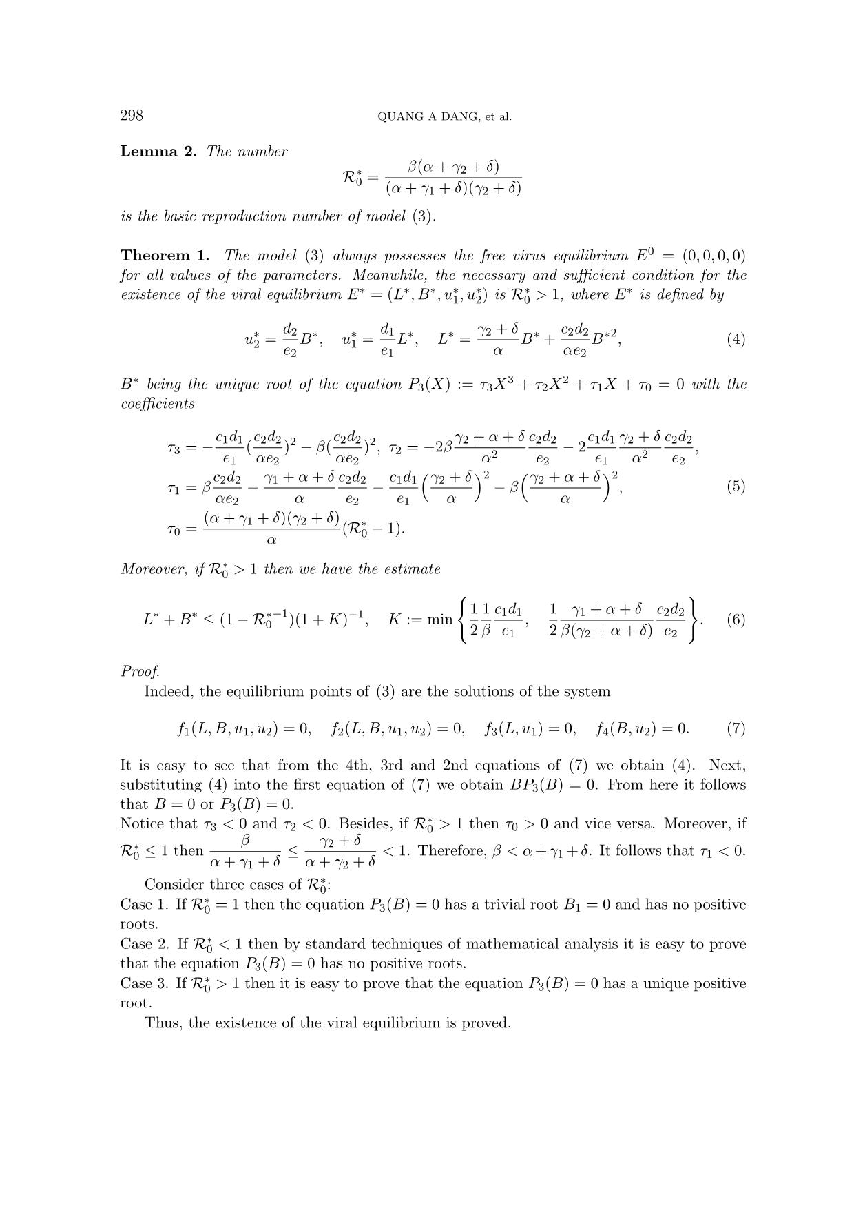
Theorem 1. The model (3) always possesses the free virus equilibrium E0 = (0, 0, 0, 0)
for all values of the parameters. Meanwhile, the necessary and sufficient condition for the
 ∗ ∗ ∗ ∗ ∗ ∗ ∗
existence of the viral equilibrium E = (L ,B , u1, u2) is R0 > 1, where E is defined by
 ∗ d2 ∗ ∗ d1 ∗ ∗ γ2 + δ ∗ c2d2 ∗2
 u2 = B , u1 = L ,L = B + B , (4)
 e2 e1 α αe2
 ∗ 3 2
B being the unique root of the equation P3(X) := τ3X + τ2X + τ1X + τ0 = 0 with the
coefficients
 c1d1 c2d2 2 c2d2 2 γ2 + α + δ c2d2 c1d1 γ2 + δ c2d2
 τ3 = − ( ) − β( ) , τ2 = −2β 2 − 2 2 ,
 e1 αe2 αe2 α e2 e1 α e2
 c2d2 γ1 + α + δ c2d2 c1d1 γ2 + δ 2 γ2 + α + δ 2
 τ1 = β − − − β , (5)
 αe2 α e2 e1 α α
 (α + γ + δ)(γ + δ)
 τ = 1 2 (R∗ − 1).
 0 α 0
 ∗
Moreover, if R0 > 1 then we have the estimate
 ( )
 ∗ ∗ ∗−1 −1 1 1 c1d1 1 γ1 + α + δ c2d2
 L + B ≤ (1 − R0 )(1 + K) ,K := min , . (6)
 2 β e1 2 β(γ2 + α + δ) e2
Proof.
 Indeed, the equilibrium points of (3) are the solutions of the system
 f1(L, B, u1, u2) = 0, f2(L, B, u1, u2) = 0, f3(L, u1) = 0, f4(B, u2) = 0. (7)
It is easy to see that from the 4th, 3rd and 2nd equations of (7) we obtain (4). Next,
substituting (4) into the first equation of (7) we obtain BP3(B) = 0. From here it follows
that B = 0 or P3(B) = 0.
 ∗
Notice that τ3 1 then τ0 > 0 and vice versa. Moreover, if
 ∗ β γ2 + δ
R0 ≤ 1 then ≤ < 1. Therefore, β < α + γ1 + δ. It follows that τ1 < 0.
 α + γ1 + δ α + γ2 + δ
 ∗
 Consider three cases of R0:
 ∗
Case 1. If R0 = 1 then the equation P3(B) = 0 has a trivial root B1 = 0 and has no positive
roots.
 ∗
Case 2. If R0 < 1 then by standard techniques of mathematical analysis it is easy to prove
that the equation P3(B) = 0 has no positive roots.
 ∗
Case 3. If R0 > 1 then it is easy to prove that the equation P3(B) = 0 has a unique positive
root.
 Thus, the existence of the viral equilibrium is proved.
 A COMPUTER VIRUS PROPAGATION MODEL 299
 Next, consecutively multiplying the first and the second equations of (7) by γ2 + α + δ
and γ1 + α + δ respectively, and adding side-by-side of the resulting equations we obtain
 ∗ ∗ 2 ∗ ∗ ∗
 − β(γ2 + α + δ)(L + B ) + (γ2 + δ)(γ1 + α + δ)(R0 − 1)(L + B )
 ∗ ∗ ∗ ∗
 − (γ2 + α + δ)c1u1L − (γ1 + α + δ)c2u2B = 0.
 It follows that
 " #
 ∗ ∗ ∗−1 1 ∗ ∗ γ1 + α + δ ∗ ∗ 1
 L + B = (1 − R0 ) − c1u1L + c2u2B ∗ ∗ .
 β β(γ2 + α + δ) L + B
 ∗ ∗
 ∗ d1L ∗ d2B 2 2
Taking into account u1 = , u2 = and using the simple inequality 2(L + B ) ≥
 e1 e2
(L + B)2 we obtain
 1 ∗ ∗ γ1 + α + δ ∗ ∗ 1 c1d1 ∗2 γ1 + α + δ c2d2 ∗2 ∗ ∗ 2
 c1u1L + c2u2B = L + B ≥ K(L + B ) .
 β β(γ2 + α + δ) β e1 β(γ2 + α + δ) e2
Therefore,
 ∗ ∗ ∗−1 ∗ ∗
 L + B ≤ (1 − R0 ) − K(L + B ).
From here it follows the inequality (6) to be proved.
Remark.
 ∗
 Suppose it is proved that if the viral equilibrium exists (R0 > 1) then it is globally stable
(this result will be established in the next section). Then, we desire L∗ + B∗ to be as small
as possible. The estimate (6) shows that it is possible to make L∗ + B∗ arbitrarily small
by making K sufficiently large. This may be achieved because K depends on the control
variables (see Table 1 in Section 4.) Particularly, when K → ∞ then E∗ moves to the
origin, i.e., the viral equilibrium vanishes. In that time, for the model (2) we always have
 −1
L∗ + B∗ = 1 − R0 (see [16]). This fact indirectly confirms the important role of the control
variables.
 3. GLOBAL STABILITY OF THE MODEL WITH FEEDBACK
 CONTROLS
 In this section, we will establish the global stability property of the model (3).
3.1. Global stability of the equilibrium E0
 The following theorem is of the global stability of E0 established with the use of a linear
Lyapunov function.
Theorem 2. The equilibrium point E0 is globally asymptotically stable of (3) in Ω∗ if
 ∗
R0 ≤ 1.
300 QUANG A DANG, et al.
Proof.
 ∗
 We define the Lyapunov function V :Ω → R+ by
 1 α + γ2 + δ 2 1 α + γ1 + δ 2
 V (L, B) = (α + γ2 + δ)L + (α + γ1 + δ)B + c1u1 + c2u2.
 2 d1 2 d2
The time derivative of the function V (L, B) along the trajectories of system (3) is
 dV
 = [β(α + γ + δ) − (γ + δ)(α + γ + δ)]B + [β(α + γ + δ) − (γ + δ)(α + γ + δ)]L
 dt 2 2 1 2 2 1
 2 α + γ2 + δ 2 α + γ1 + δ 2
 − β(α + γ2 + δ)(L + B) − e1c1u1 − e2c2u2
 d1 d2
 ≤ [β(α + γ2 + δ) − (γ2 + δ)(α + γ1 + δ)]B + [β(α + γ2 + δ) − (γ2 + δ)(α + γ1 + δ)]L
 ∗
 = (γ2 + δ)(α + γ1 + δ)(R0 − 1)(L + B).
Obviously, dV /dt < 0 strictly for all (L, B) ∈ Ω∗ except for the equilibrium E0, where
dV /dt = 0. Hence, the function V satisfies Lyapunov’s asymptotic stability theorem [8], and
 0
the equilibrium point E of system (3) is globally stable.
3.2. Numerical simulations for investigating global stability of the positive equi-
 librium point
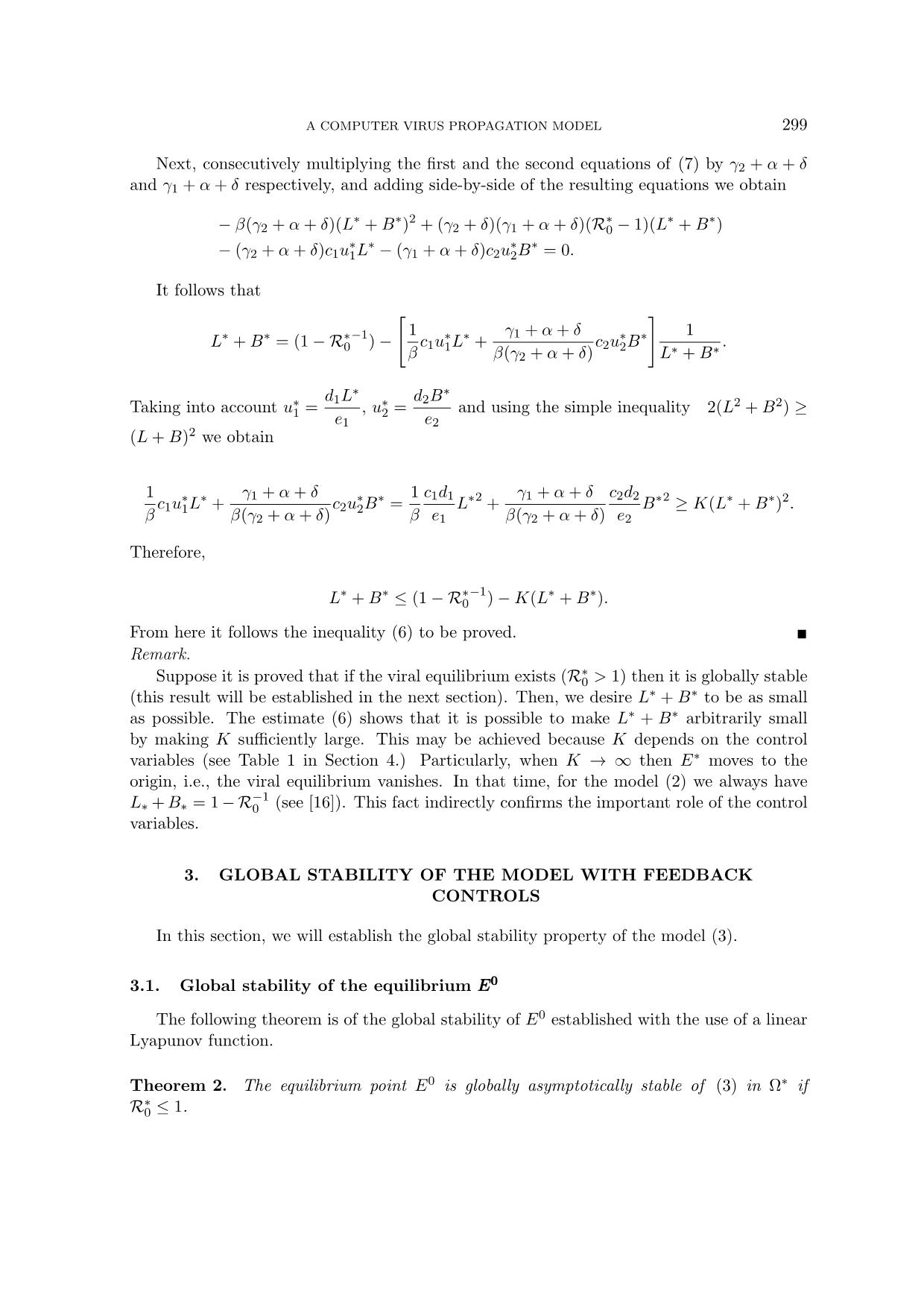
 In this subsection, some numerical simulations are performed to investigate the global
stability of the positive equilibrium point E∗. For this purpose, we consider model (3) with
the parameters
 α = 0.1, β = 0.8, δ = 0.2, γ1 = 0.1, γ2 = 0.2.
 ∗
In this case, we have R0 = 2.5 > 1. We select the control variables as follows
 c1 = 1, c2 = 2, d1 = 1, d2 = 1.25, e1 = 2, e2 = 5.
Consequently, the unique positive equilibrium point is given by
 E∗ = (0.3413, 0.0778, 0.1707, 0.0194).
The solution of the model (3) with several initial values are depicted in Figure 1. From this
figure it is seen that E∗ is globally stable. It should be emphasized that all other numerical
simulations, including those in Section 4, give similar results. This means the global stability
of E∗ is observed.
 A COMPUTER VIRUS PROPAGATION MODEL 301
 0.5 0.8
 0.4
 0.6
 0.3
 0.4
 0.2
 0.2
 0.1
 0 0
 0 5 10 15 20 0 5 10 15 20
 t t
 1 1
 0.8 0.8
 0.6 0.6
 0.4 0.4
 0.2 0.2
 0 0
 0 5 10 15 20 0 5 10 15 20
 t t
Figure 1. Solution of model (3) by the classical fourth order Runge-Kutta method (L-blue, B−red,
u1-green, u2-cyan)
 4. NUMERICAL SIMULATIONS
 In this Section, we perform some numerical simulations to show the influence of control
variables.
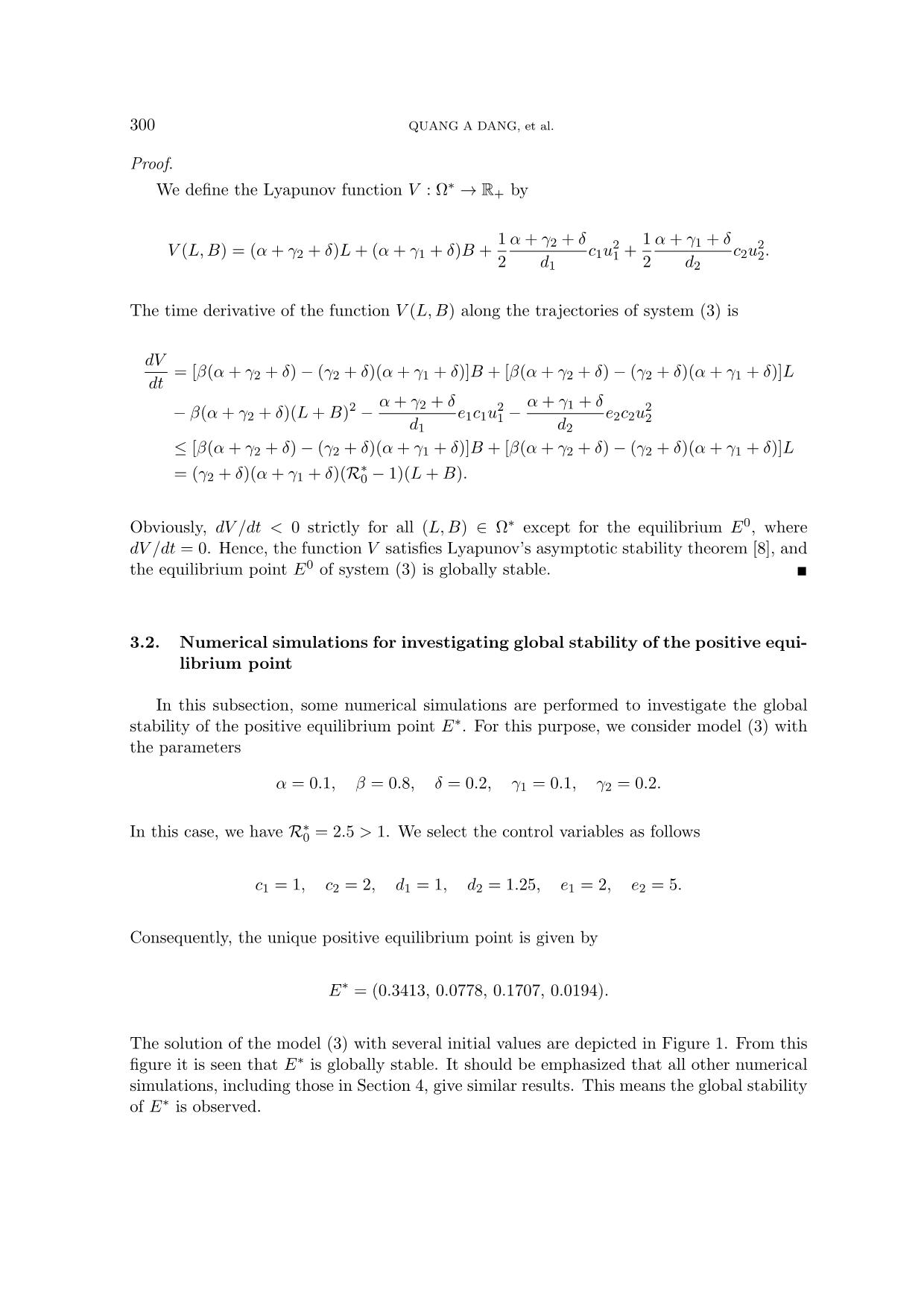
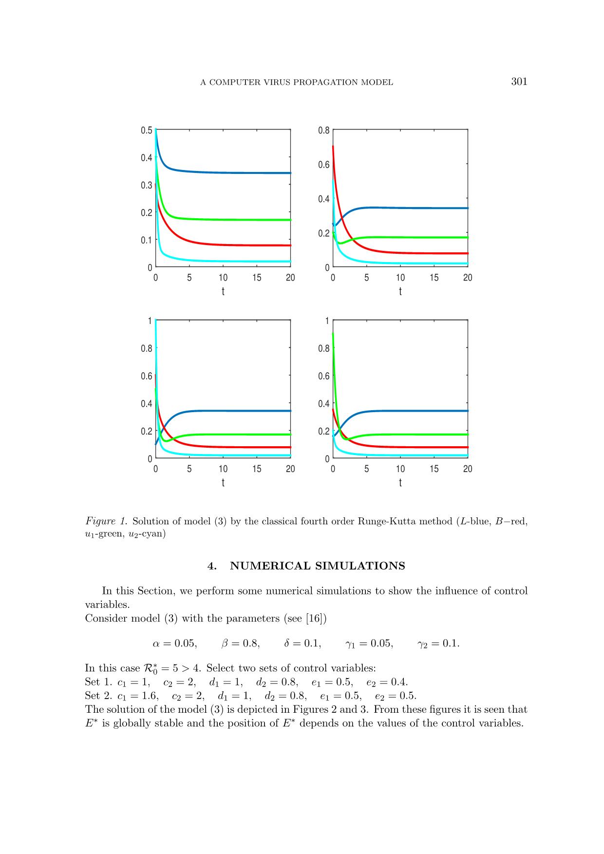
Consider model (3) with the parameters (see [16])
 α = 0.05, β = 0.8, δ = 0.1, γ1 = 0.05, γ2 = 0.1.
 ∗
In this case R0 = 5 > 4. Select two sets of control variables:
Set 1. c1 = 1, c2 = 2, d1 = 1, d2 = 0.8, e1 = 0.5, e2 = 0.4.
Set 2. c1 = 1.6, c2 = 2, d1 = 1, d2 = 0.8, e1 = 0.5, e2 = 0.5.
The solution of the model (3) is depicted in Figures 2 and 3. From these figures it is seen that
E∗ is globally stable and the position of E∗ depends on the values of the control variables.
302 QUANG A DANG, et al.
 0.7
 L
 B
 u
 0.6 1
 u
 2
 0.5
 0.4
 0.3
 0.2
 0.1
 0
 0 5 10 15 20 25 30
 t
 Figure 2. The solutions of model (3) for Set 1: K = 1.25, E∗ = (0.2352, 0.0347, 0.4703, 0.0694)
 0.8
 L
 B
 u
 0.7 1
 u
 2
 0.6
 0.5
 0.4
 0.3
 0.2
 0.1
 0
 0 5 10 15 20 25 30
 t
 Figure 3. The solutions of model (3) for Set 2: K = 1.6, E∗ = (0.1714, 0.0292, 0.3428, 0.0465)
 We draw a special attention to the fact that the model (2) has E∗ = (0.64, 0.16), meanw-
hile the values of E∗ of the model (3) for Set 1 and Set 2 are (0.2352, 0.0347, 0.4703, 0.0694)
(K = 1.25) and E∗ = (0.1714, 0.0292, 0.3428, 0.0465) (K = 1.6), respectively. From that
we see that the control variables have active influence on the position of equilibrium points.
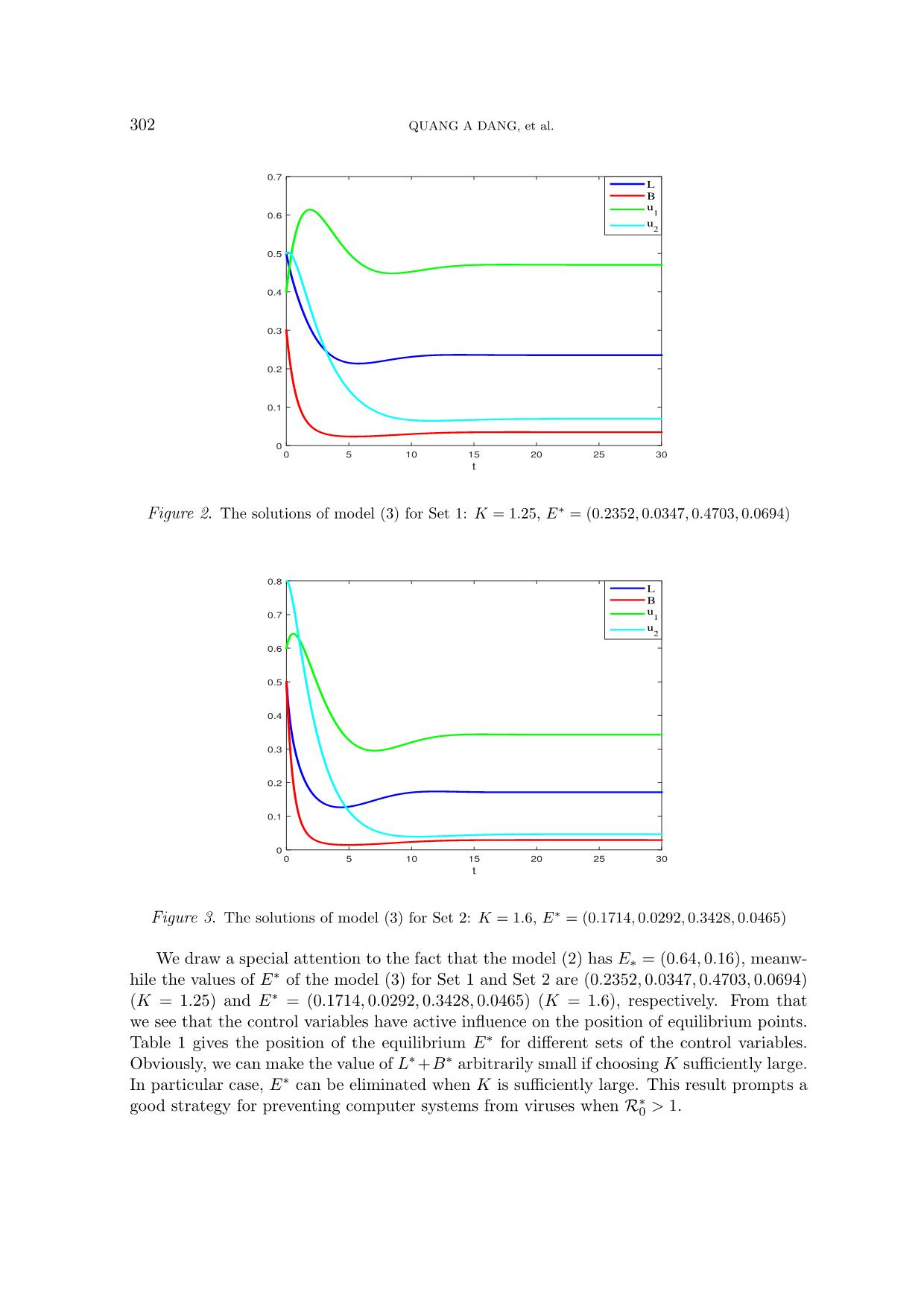
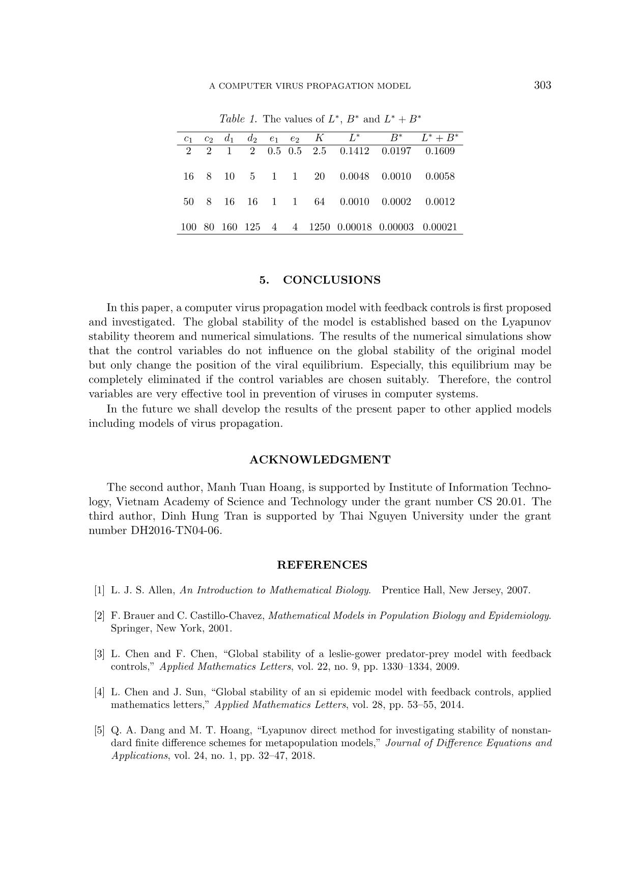
Table 1 gives the position of the equilibrium E∗ for different sets of the control variables.
Obviously, we can make the value of L∗ +B∗ arbitrarily small if choosing K sufficiently large.
In particular case, E∗ can be eliminated when K is sufficiently large. This result prompts a
 ∗
good strategy for preventing computer systems from viruses when R0 > 1.
 A COMPUTER VIRUS PROPAGATION MODEL 303
 Table 1. The values of L∗, B∗ and L∗ + B∗
 ∗ ∗ ∗ ∗
 c1 c2 d1 d2 e1 e2 KL B L + B
 2 2 1 2 0.5 0.5 2.5 0.1412 0.0197 0.1609
 16 8 10 5 1 1 20 0.0048 0.0010 0.0058
 50 8 16 16 1 1 64 0.0010 0.0002 0.0012
 100 80 160 125 4 4 1250 0.00018 0.00003 0.00021
 5. CONCLUSIONS
 In this paper, a computer virus propagation model with feedback controls is first proposed
and investigated. The global stability of the model is established based on the Lyapunov
stability theorem and numerical simulations. The results of the numerical simulations show
that the control variables do not influence on the global stability of the original model
but only change the position of the viral equilibrium. Especially, this equilibrium may be
completely eliminated if the control variables are chosen suitably. Therefore, the control
variables are very effective tool in prevention of viruses in computer systems.
 In the future we shall develop the results of the present paper to other applied models
including models of virus propagation.
 ACKNOWLEDGMENT
 The second author, Manh Tuan Hoang, is supported by Institute of Information Techno-
logy, Vietnam Academy of Science and Technology under the grant number CS 20.01. The
third author, Dinh Hung Tran is supported by Thai Nguyen University under the grant
number DH2016-TN04-06.
 REFERENCES
 [1] L. J. S. Allen, An Introduction to Mathematical Biology. Prentice Hall, New Jersey, 2007.
 [2] F. Brauer and C. Castillo-Chavez, Mathematical Models in Population Biology and Epidemiology.
 Springer, New York, 2001.
 [3] L. Chen and F. Chen, “Global stability of a leslie-gower predator-prey model with feedback
 controls,” Applied Mathematics Letters, vol. 22, no. 9, pp. 1330–1334, 2009.
 [4] L. Chen and J. Sun, “Global stability of an si epidemic model with feedback controls, applied
 mathematics letters,” Applied Mathematics Letters, vol. 28, pp. 53–55, 2014.
 [5] Q. A. Dang and M. T. Hoang, “Lyapunov direct method for investigating stability of nonstan-
 dard finite difference schemes for metapopulation models,” Journal of Difference Equations and
 Applications, vol. 24, no. 1, pp. 32–47, 2018.
304 QUANG A DANG, et al.
 [6] Q. A. Dang, M. T. Hoang, D. Y. Trejos, and J. C. Valverde, “Feedback control variables to
 restrain the babesiosis disease,” Mathematical Methods in the Applied Sciences, vol. 42, pp.
 7517–7527, 2019.
 [7] H. L. Li, L. Zhang, Z. Teng, Y. L. Jiang, and A. Muhammadhaji, “Global stability of an si
 epidemic model with feedback controls in a patchy environment,” Applied Mathematics and
 Computation, vol. 321, pp. 372–384, 2018.
 [8] A. M. Lyapunov, General Problem of the Stability of Motion. Taylor & Francis, London, 1992.
 [9] M. R. Parsaei, R. Javidan, N. S. Kargar, and H. S. Nik, “On the global stability of an epidemic
 model of computer viruses,” Theory in Biosciences, vol. 136, pp. 169–178, 2017.
[10] J. R. C. Piqueira and V. O. Araujo, “A modified epidemiological model for computer viruses,”
 Applied Mathematics and Computation, vol. 213, pp. 355–360, 2009.
[11] Y. Shang, “Global stability of disease-free equilibria in a two-group si model with feedback
 control,” Nonlinear Analysis: Modelling and Control, vol. 20, pp. 501–508, 2015.
[12] J. P. Tripathi and S. Abbas, “Global dynamics of autonomous and nonautonomous si epidemic
 models with nonlinear incidence rate and feedback controls,” Nonlinear Dynamics, vol. 86, pp.
 337–351, 2016.
[13] P. van den Driessche and J. Watmough, “Reproduction numbers and sub-threshold endemic
 equilibria for compartmental models of disease transmission,” Mathematical Biosciences, vol.
 180, pp. 29–48, 2002.
[14] L. Yang, X. Yang, L. Wen, and J. Liu, “A novel computer virus propagation model and its
 dynamics,” International Journal of Computer Mathematics, vol. 89, pp. 2307–2314, 2012.
[15] L. X. Yang and X. Yang, “A new epidemic model of computer viruses,” Communications in
 Nonlinear Science and Numerical Simulation, vol. 19, no. 9, pp. 1935–1944, 2014.
[16] L. X. Yang, X. Yang, Q. Zhu, and L. Wen, “A computer virus model with graded cure rates,”
 Nonlinear Analysis: Real World Applications, vol. 14, pp. 414–422, 2013.
[17] X. Yang, B. K. Mishra, and Y. Liu, “Computer virus: theory, model, and methods,” Discrete
 Dynamics in Nature and Society, pp. 473–508, 2012.
 Received on September 30, 2020
 Revised on October 21, 2020
File đính kèm:
 global_dynamics_of_a_computer_virus_propagation_model_with_f.pdf

